Introduction
RNA sequencing (RNA-Seq) stands as one of the most prevalent forms of next-generation sequencing in contemporary bioinformatics research. Bulk-RNA-Seq, a technique that offers a comprehensive overview of gene expression by pooling RNA isolated from many cells, was the predominant technique until relatively recently. Despite the advent of single-cell RNA-Seq (scRNA-Seq) technologies, offering the ability to dissect the transcriptomic landscape resolved spatially within tissues at the individual cellular level, bulk RNA-Seq (and ultra-low input variants) continue to hold significant value. These methods not only remain essential tools in biomedical studies for their efficiency, cost-effectiveness, and ability to generate robust datasets across a wide range of sample types, but they’re also the obvious place to start learning transcriptomics before moving into more advanced contemporary techniques.
Virtually all of the myriad RNA-Seq analysis tutorials available online start with a counts matrix from an open-access experiment. In an attempt to be a little different, I want to start at the very beginning and try to demystify the raw data analysis as well.
This series of tutorials aims to navigate the entire bulk RNA-Seq data analysis journey from raw reads to publication-ready figures for differential expression (DE) testing and gene set enrichment analyses. My aim is not to delve into the theory, or the possibilities and complexities an experienced bioinformatician might consider at each stage of the workflow, but to show the uninitiated the basics of each step in the process. I will focus on the streamlined essentials and what I think is the most effective way to setup and run all the tools required to get the results that most biologists running a bulk RNA-Seq will want.
To follow along with this series you will need:
- PC or Laptop with an internet connection
- R and RStudio installed on your local machine
- High-Performance Computer e.g., institutional cluster (Tutorial 1 only)
If you do not have access to an institutional high-performance computing or cloud computing account or just want to learn the processed data analysis, feel free to skip to the second tutorial in the series. I will be provided some instructions for installing R and RStudio in the software setup section of the second tutorial.
My hope is that by the end of this series, anyone following along will have met the following learning outcomes:
- Master basic setup and operation of nf-core for bioinformatic analysis
- Execute the nf-core/rnaseq pipeline for FASTQ file analysis
- Transfer transcript count data into R for processing
- Conduct exploratory analysis and normalisation of transcript count data
- Perform quality control to identify outliers, batch effects, and sample discrepancies
- Apply DESeq2 for differential expression testing
- Generate and interpret key visualisations for experimental results
- Utilise annotation packages for biological database queries
- Execute gene set enrichment and over-representation analyses
The Bulk RNA-Seq Analysis Pipeline
Historically, demonstrating raw data analysis would have been a mammoth task, necessitating learning relatively advanced BASh scripting and pipeline development to even get started. Luckily, the bioinformatic processing of raw next generation sequencing data has never been so easy thanks to a revolutionary bioinformatics community project: nf-core.
Beginning in early 2018, the nf-core project aims to establish a collection of high-quality Nextflow pipelines for bioinformatics. Nextflow itself is a workflow tool that enables scalable and reproducible scientific workflows using software containers, facilitating pipeline development in a portable and efficient manner. The nf-core project builds on this by providing a suite of ready-to-use workflows that cover a wide range of genomic and bioinformatic analysis scenarios, all developed and maintained by a consortium of experts in the field.
The pipelines comprising nf-core are designed to be used across a variety of compute infrastructures while adhering to best practices in both software development and bioinformatics. They are subjected to rigorous testing, ensuring they meet the highest standards of reliability and efficiency. This has led to their widespread adoption by most UK institutions and core facilities active in bioinformatics research.
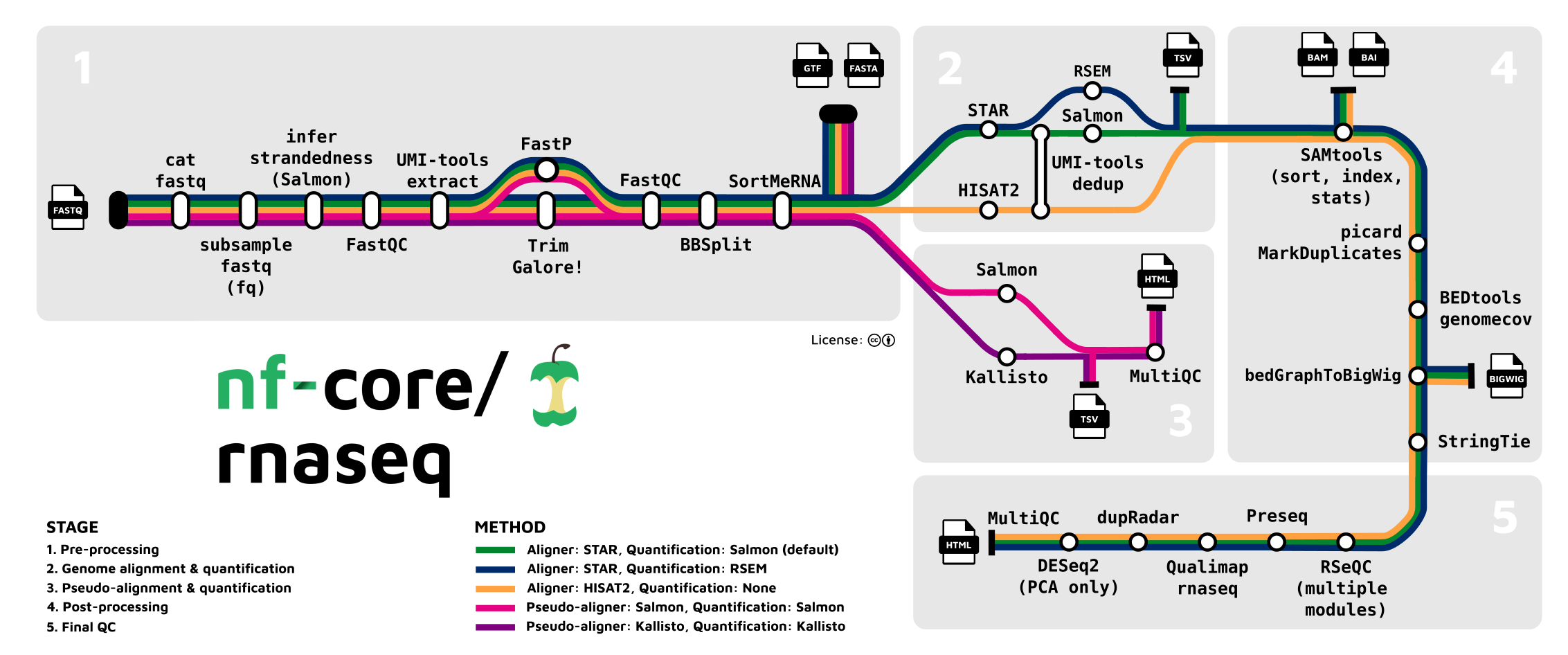
The pipeline that we will be using in the first part of this tutorial series is the nf-core/rnaseq, an RNA sequencing analysis pipeline that uses gold-standard tools such as STAR, RSEM and Salmon to provide both gene transcript or isoform counts as well as extensive quality control.
If we are going to run this beast, the first thing that we will need to do is setup and get some data. Let’s get into it!
Software Setup
In order to streamline the integration of multiple analytical tools and ensure reproducibility between analyses, nf-core pipelines utilise the built-in support for containerisation or software packaging that Nextflow offers. This means that you will need some form of containerisation software e.g., Docker / Singularity / Apptainer installed on your HPC system. You are also going to need Java. A guide on how to do this is outside of the scope of this tutorial so consult your HPC documentation or contact a system admin to check availability or arrange installation. The system I am using to write this tutorial has Singularity / Apptainer installed.
Given the breadth of high-performance compute infrastructure, workflow managers, and specific ways that these systems might have been configured across research institutions, providing a tutorial on how to undertake the setup process for each different scenario would be almost impossible. If someone hasn’t already setup Nextflow and nf-core for you at your institution for you, detailed guidance on how to do this can be found in the nf-core documentation. You can check whether an institutional configuration profile exists where you work by checking the list available here. Don’t worry if you don’t have an institutional nf-core configuration profile, this isn’t mission critical, and I will show a quick and easy work-around for this later on.
The general series of steps required for getting Nextflow and nf-core setup are as follows:
- Login to your HPC account and request an interactive session
- Install and configure a package manager such as Conda
- Setup a Nextflow and nf-core analysis environment
- Setup your project
- Configure and execute the pipeline run
You can find a good, streamlined implementation of these steps in the guide I wrote for the University of Sheffield Bioinformatics Core during my time working there at this link.
The advantages of using the miniconda method that I am going to show to get Nextflow, nf-core, and virtually all of their dependencies installed is that it is quick to do and almost identical no matter where you want to run these pipelines.
It might be that you already have anaconda or miniconda available on your HPC system. If not, it is likely that you can easily install this as a TCL module as shown in the guide linked above. Check your institutional documentation or contact a system admin to check. A relatively detailed guide to conda setup can be found in part 1 and part 2 of the series that I wrote on this topic a couple of years ago.
Once you have made sure conda is installed on your system and your channel priority configured, the next thing to do is create a conda environment into which we can install nextflow, nf-core and all their requisite dependencies.
# load conda module
module load miniconda

# make the "nf_env" environment
conda create --name nf_env nextflow nf-core

# activate the environment (some systems might require source activate here)
conda activate nf_env
Once that’s done we can run a couple of commands to make sure that nextflow is installed and working. First run the following nextflow command:
# test the environment is working
nextflow info
You should see output resembling that shown here:
Version: 23.10.1 build 5891
  Created: 12-01-2024 22:01 UTC (22:01 BST)
  System: Linux 3.10.0-1160.105.1.el7.x86_64
  Runtime: Groovy 3.0.19 on OpenJDK 64-Bit Server VM 21-internal-adhoc.conda.src
  Encoding: UTF-8 (ANSI_X3.4-1968)
We can then run a simple “hello world” pipeline to check nextflow and the containerisation software are working correctly:
# test functionality
nextflow run hello
The output should look something like this:
N E X T F L O W  ~  version 23.10.1
Launching `https://github.com/nextflow-io/hello` [zen_carlsson] DSL2 - revision: 1d71f857bb [master]
executor >  local (4)
[a7/36b0a8] process > sayHello (3) [100%] 4 of 4 ✔
Hola world!

Ciao world!

Bonjour world!

Hello world!
Finally, deactivate the conda environment now that everything is confirmed to be working.
# deactivate the "nf_env" environment
conda deactivate

# deactivate conda
module unload miniconda
Once that’s done, we can setup our project folders.
Project Setup
This is a somewhat opinionated guide i.e., it follows the system that I have developed, so we are going to use the same project directory hierarchy I use for almost all of my projects. To set this up, we can run a simple one-line BASh command wherever you want the project directory to be created as follows:
# make the project directory hierarchy
mkdir -p ./2024_05_01_rnaseq_end_to_end/{data/{raw,reference,sample_sheet},results,src/{nf_config,nf_params,shell}}
Easy. Now we are ready to get the data we will use for the tutorial.
Data Acquisition
The data set that we will use for this tutorial comes from the publication Induction of fibroblast senescence generates a non-fibrogenic myofibroblast phenotype that differentially impacts on cancer prognosis.
Cancer associated fibroblasts characterized by an myofibroblastic phenotype play a major role in the tumour microenvironment, being associated with poor prognosis. We found that this cell population is made in part by senescent fibroblasts in vivo. As senescent fibroblasts and myofibroblasts have been shown to share similar tumour promoting functions in vitro we compared the transcriptomes of these two fibroblast types and performed RNA-seq of human foetal foreskin fibroblasts 2 (HFFF2) treated with 2ng/ml TGF-beta-1 to induce myofibroblast differentiation or 10Gy gamma irradiation to induce senescence. We isolated RNA 7 days upon these treatments changing the medium 3 days before the RNA extraction.
The various FASTQ files for this project can be downloaded from the PRJEB8248 project page on the European Nucleotide Archive (ENA). The easiest way to download all these files at once is using a small shell script such as the one shown below. For convenience, you can download the template shell script from here and saved it within the shell folder of the project src directory.
#!/bin/bash

# specify the raw data directory path
RAW_DIR="/path/to/project/yyyy_mm_dd_rnaseq_end_to_end/data/raw"

# variable of links to files for download
LINKS="
ftp://ftp.sra.ebi.ac.uk/vol1/run/ERR732/ERR732903/3_IR_BC_5.fastq.gz
ftp://ftp.sra.ebi.ac.uk/vol1/run/ERR732/ERR732905/6_IR_BC_12.fastq.gz
ftp://ftp.sra.ebi.ac.uk/vol1/run/ERR732/ERR732904/7_CTR_BC_13.fastq.gz
ftp://ftp.sra.ebi.ac.uk/vol1/run/ERR732/ERR732902/5_TGF_BC_7.fastq.gz
ftp://ftp.sra.ebi.ac.uk/vol1/run/ERR732/ERR732909/9_IR_BC_15.fastq.gz
ftp://ftp.sra.ebi.ac.uk/vol1/run/ERR732/ERR732907/2_TGF_BC_4.fastq.gz
ftp://ftp.sra.ebi.ac.uk/vol1/run/ERR732/ERR732906/1_CTR_BC_2.fastq.gz
ftp://ftp.sra.ebi.ac.uk/vol1/run/ERR732/ERR732908/8_TGF_BC_14.fastq.gz
ftp://ftp.sra.ebi.ac.uk/vol1/run/ERR732/ERR732901/4_CTR_BC_6.fastq.gz
"

# download files
for LINK in $LINKS; do

  wget -nc $LINK -P $RAW_DIR

done
Be sure to modify the template so that the string assigned to the $RAW_DIR variable points to the raw data folder within the data directory e.g., /mnt/parscratch/users/${USER}/2024_05_01_rnaseq_end_to_end/data/raw. Once you have done this, you can run it with the following command (again making sure to edit the placeholder path):
bash /path/to/project/yyyy_mm_dd_rnaseq_end_to_end/src/shell/PRJEB8248_fastq_download.sh
The metadata sheet for this project on ENA details the experimental conditions and the nature of the various FASTQ files that we will be using in the first part of this tutorial series. You can be download a CSV version of the metadata sheet directly from here and place this into the sample_sheet directory within the project data folder. We will need this later in this series when we are working in R.
Once the raw data files and the metadata sheet have been downloaded, we need to get our reference genome FASTA and GTF files. In this instance, both files can be downloaded from Ensembl. The easiest way to download both files at once is using another shell script such as the one shown below. For convenience, you can download the template shell script from here and ensure it is placed within the shell folder of the project src directory.
#!/bin/bash

# specify the reference directory path
REF_DIR="/path/to/project/yyyy_mm_dd_rnaseq_end_to_end/data/reference"

# specify reference genome version - changes regularly
VERSION="111"

# download files
wget "ftp://ftp.ensembl.org/pub/release-${VERSION}/fasta/homo_sapiens/dna/Homo_sapiens.GRCh38.dna_sm.primary_assembly.fa.gz" -P ${REF_DIR}
wget "ftp://ftp.ensembl.org/pub/release-${VERSION}/gtf/homo_sapiens/Homo_sapiens.GRCh38.${VERSION}.gtf.gz" -P ${REF_DIR}

# decompress .gz archives
gzip -d "${REF_DIR}/Homo_sapiens.GRCh38.dna_sm.primary_assembly.fa.gz"
gzip -d "${REF_DIR}/Homo_sapiens.GRCh38.${VERSION}.gtf.gz"
As before, be sure to modify the template so that the string assigned to the $REF_DIR variable points to the reference folder within the data directory of your project. For example, /mnt/parscratch/users/${USER}/2024_05_01_rnaseq_end_to_end/data/reference. Once you have done this, you can run it with a bash command as before.
bash /path/to/project/yyyy_mm_dd_rnaseq_end_to_end/src/shell/GRCh38p14_ref_download.sh
The last thing we need to do in preparation is to setup a sample sheet for the files. A detailed guide on how to do this for most nf-core pipelines can be found on the pipeline document pages under the usage tab. For the nf-core/rnaseq pipeline the sample sheet requirements can be viewed here.
As we have a one file containing single end reads for each sample, the sample sheet layout is relatively simple and only requires the sample name, full path to each respective file and the strandedness on the same line. The read technology and strandedness are detailed in the experimental metadata. A template version of the sample sheet shown below can be downloaded directly from here.
sample,fastq_1,fastq_2,strandedness
1_CTR_BC_2,/path/to/project/yyyy_mm_dd_rnaseq_end_to_end/data/raw/1_CTR_BC_2.fastq.gz,,reverse
2_TGF_BC_4,/path/to/project/yyyy_mm_dd_rnaseq_end_to_end/data/raw/2_TGF_BC_4.fastq.gz,,reverse
3_IR_BC_5,/path/to/project/yyyy_mm_dd_rnaseq_end_to_end/data/raw/3_IR_BC_5.fastq.gz,,reverse
4_CTR_BC_6,/path/to/project/yyyy_mm_dd_rnaseq_end_to_end/data/raw/4_CTR_BC_6.fastq.gz,,reverse
5_TGF_BC_7,/path/to/project/yyyy_mm_dd_rnaseq_end_to_end/data/raw/5_TGF_BC_7.fastq.gz,,reverse
6_IR_BC_12,/path/to/project/yyyy_mm_dd_rnaseq_end_to_end/data/raw/6_IR_BC_12.fastq.gz,,reverse
7_CTR_BC_13,/path/to/project/yyyy_mm_dd_rnaseq_end_to_end/data/raw/7_CTR_BC_13.fastq.gz,,reverse
8_TGF_BC_14,/path/to/project/yyyy_mm_dd_rnaseq_end_to_end/data/raw/8_TGF_BC_14.fastq.gz,,reverse
9_IR_BC_15,/path/to/project/yyyy_mm_dd_rnaseq_end_to_end/data/raw/9_IR_BC_15.fastq.gz,,reverse
Be sure to place the sample sheet file within the sample_sheet folder of the data directory and then substitute the placeholder text so that each absolute path points at the correct file located in the raw folder within the data directory.
Pipeline Run Configuration
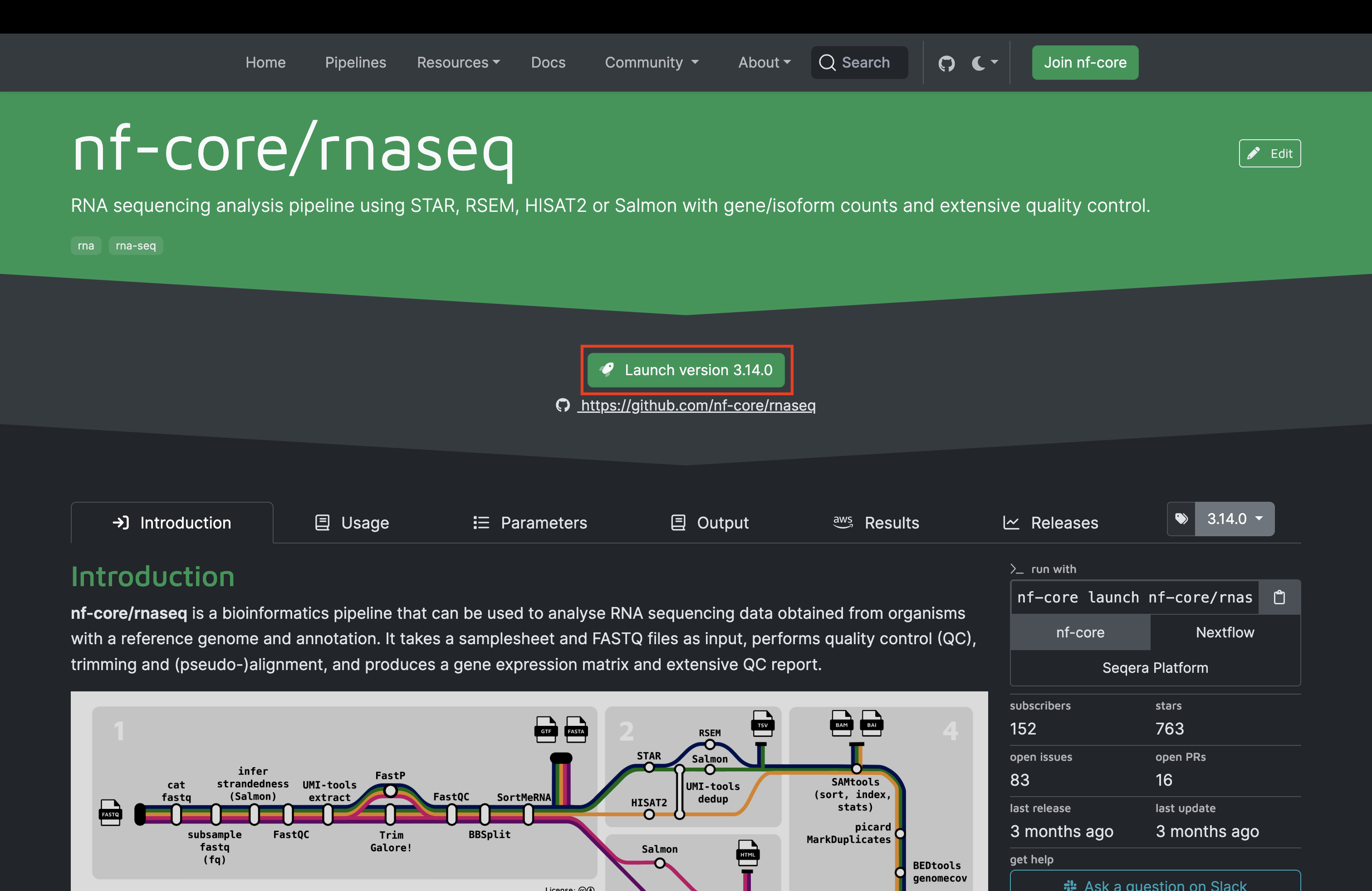
Now that we have all of the required files, we can configure the nf-core pipeline using the pipeline launcher tool on the pipeline top-level page.
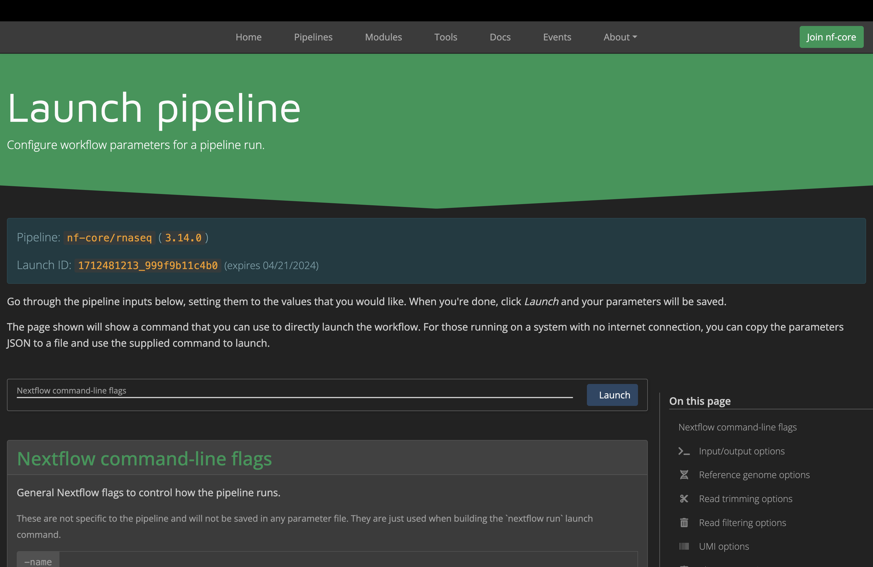
Once you hit the “Launch Pipeline” button as shown above, you will be greeted with the following page where you can provide various configuration parameters. Ensure that you follow the guide for how to enter the essential information as shown in the tutorial video.
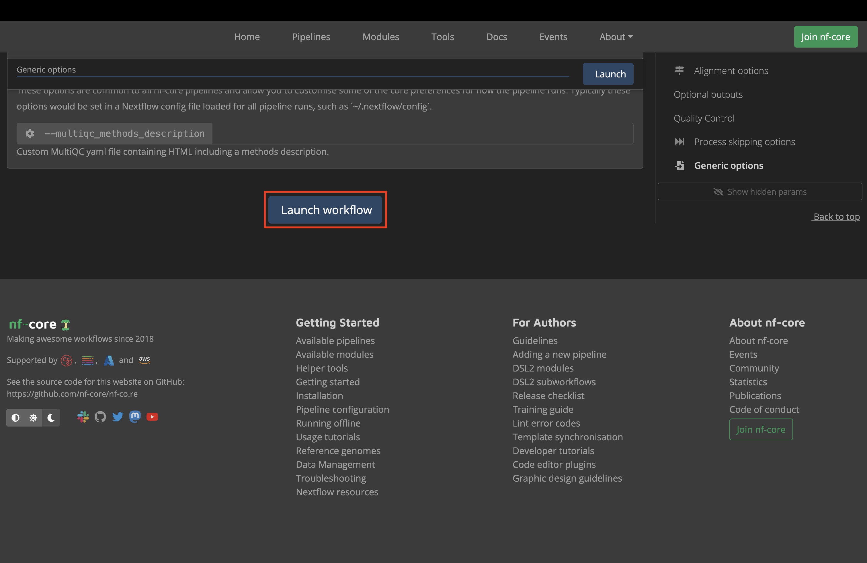
Once you get to the bottom of the page and click the blue “Launch” workflow button:
You will then be greeted with a page that looks like the one shown here:
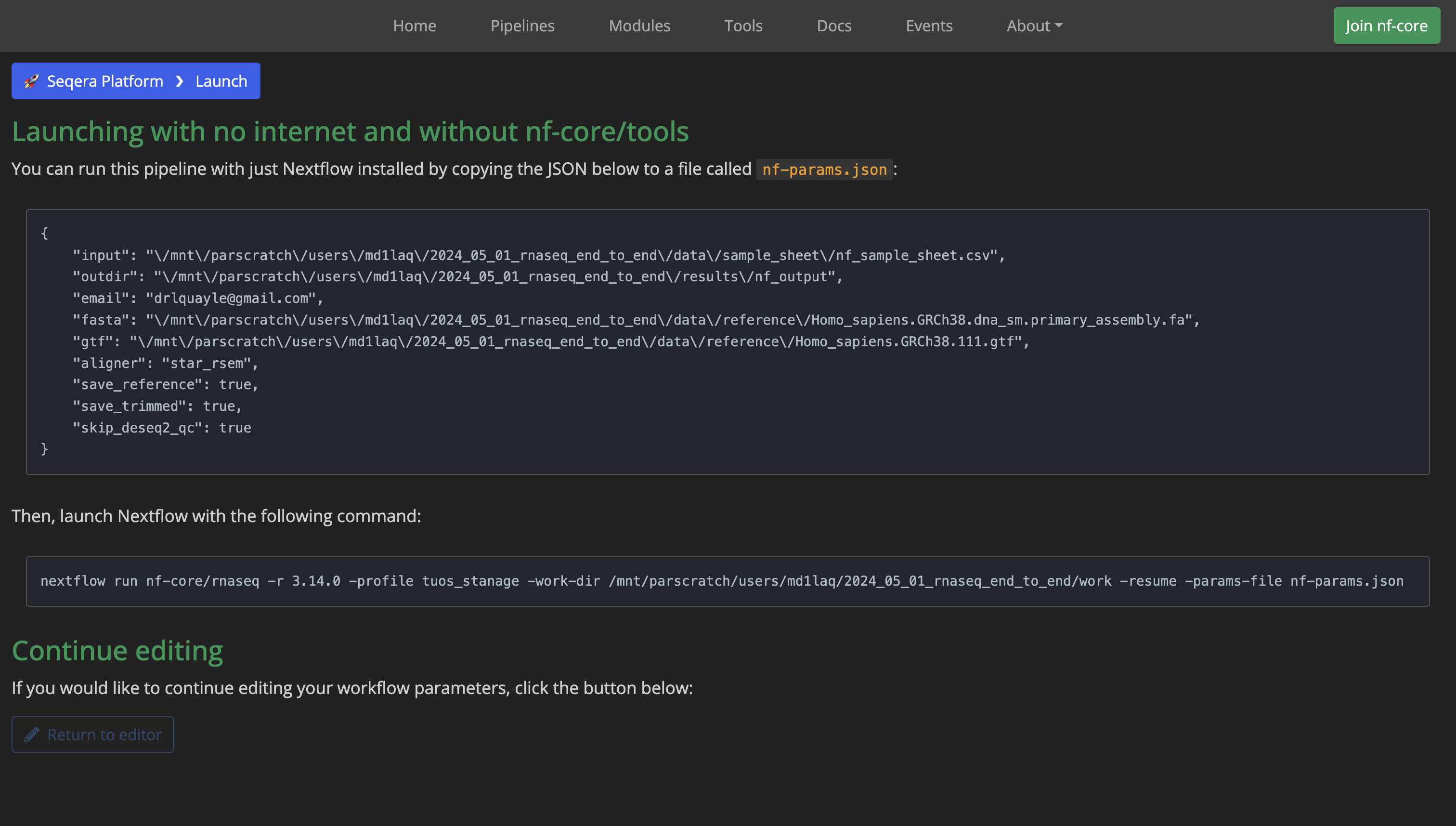
As the page instructs, open a text editor, paste in the contents of the first box and save this file as nf-params.json within the nf_params folder in the src directory.
Next, either copy the contents of the second box on the launcher page, paste these into a plain text file and format as shown below by adding in the additional bang line #!/bin/bash and other lines of code, or just download and modify this template directly from here. You should save this file as nf_run.sh inside the project shell directory.
Note: here I have used scheduler flags specific to the workflow management software installed on the HPC I am using (Slurm) but you will need to substitute and configure these flags in a manner appropriate to your system which could be running entirely different scheduer software.
#!/bin/bash

## slurm scheduler flags

# job name
#SBATCH --job-name=nfcore_rnaseq

# request resources for the job
#SBATCH --cpus-per-task=1
#SBATCH --mem=3G

# send email
#SBATCH --mail-user=a.surname@institution.ac.uk
#SBATCH --mail-type=BEGIN,END,FAIL

# output log file
#SBATCH --output=nextflow.log


## load miniconda module and activate analysis environment

module purge
module load miniconda
source activate nf_env


## export variables

# prevent java vm requesting too much memory and killing run
export NXF_OPTS="-Xms1g -Xmx2g"

# path to singularity cache
export NXF_SINGULARITY_CACHEDIR="/path/to/singularity_cache/.singularity"

# path to project directory
NF_PROJECT="/path/to/project/yyyy_mm_dd_rnaseq_end_to_end"

# project sub-directories
WORK_DIR="${NF_PROJECT}/results/nf_work"
PARAM_DIR="${NF_PROJECT}/src/nf_params"
CONF_DIR="${NF_PROJECT}/src/nf_config"


## run command

nextflow run nf-core/rnaseq \
-r 3.14.0 \
-profile institutional_profile \
-work-dir $WORK_DIR \
-params-file ${PARAM_DIR}/nf-params.json
It is important that not only that you edit the placeholder path when specifying the $NF_PROJECT variable, but also that you edit the -profile flag argument. If you happen to have an institutional configuration profile available, then you can add the appropriate profile. If not, do not despair. The solution is simple (and the reason for the seemingly unused $CONF_DIR variable in the template script). First, use the profile for the containerisation software installed on your HPC as the argument to the -profile flag e.g., -profile singularity. Next, we need to add an additional line to the run command as shown below that points at a custom configuration file for the pipeline.
# adding the -c flag for custom config
nextflow run nf-core/rnaseq \
-r 3.14.0 \
-profile institutional_profile \
-work-dir $WORK_DIR \
-params-file ${PARAM_DIR}/nf-params.json \
-c "${CONF_DIR}/custom.config"
The custom configuration file is basically an edited version of the pipeline base configuration to scale the resource requests to those available to your system, along with a function that ensures the automatic scaling of resources if the pipeline fails does not exceed the system maxima. I have included an example that you can download here.
Launch 🚀
Now that we are all setup, we need to launch the pipeline. I recommend double-checking that everything is exactly as it should be one last time. Once you’re good to go, run the appropriate batch job submission command for your scheduler, passing it your job submission script nf_run.sh, for example:
sbatch /path/to/project/yyyy_mm_dd_rnaseq_end_to_end/src/shell/nf_run.sh
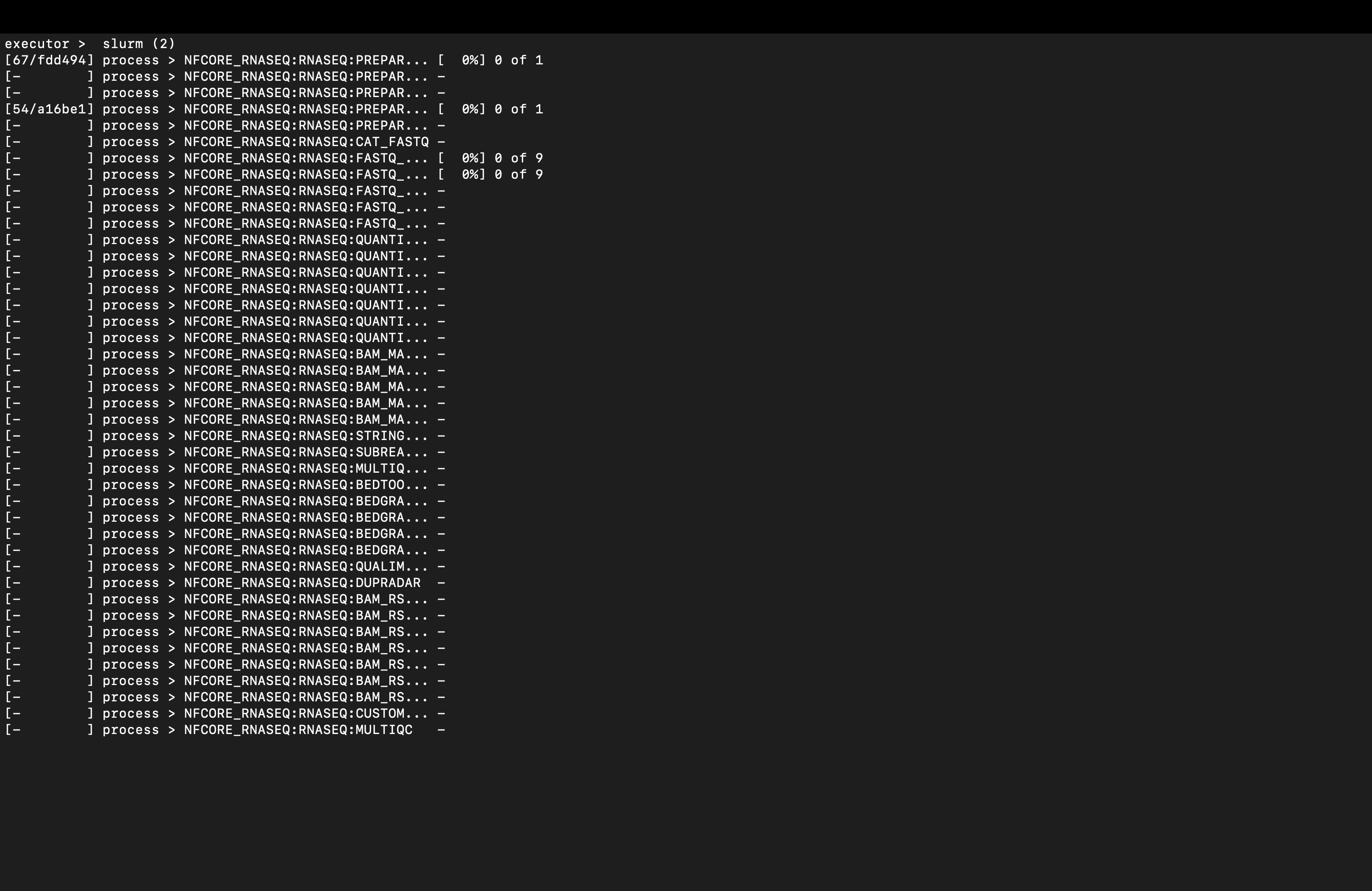
Once you receive confirmation that your job has been submitted, you can check the progress of the pipeline by consulting the nextflow.log file e.g., less /path/to/project/yyyy_mm_dd_rnaseq_end_to_end/nextflow.log. If you execute the job submission from within your project top-level, that will be the location of the log file, as this is created wherever you launch a pipeline from by default.
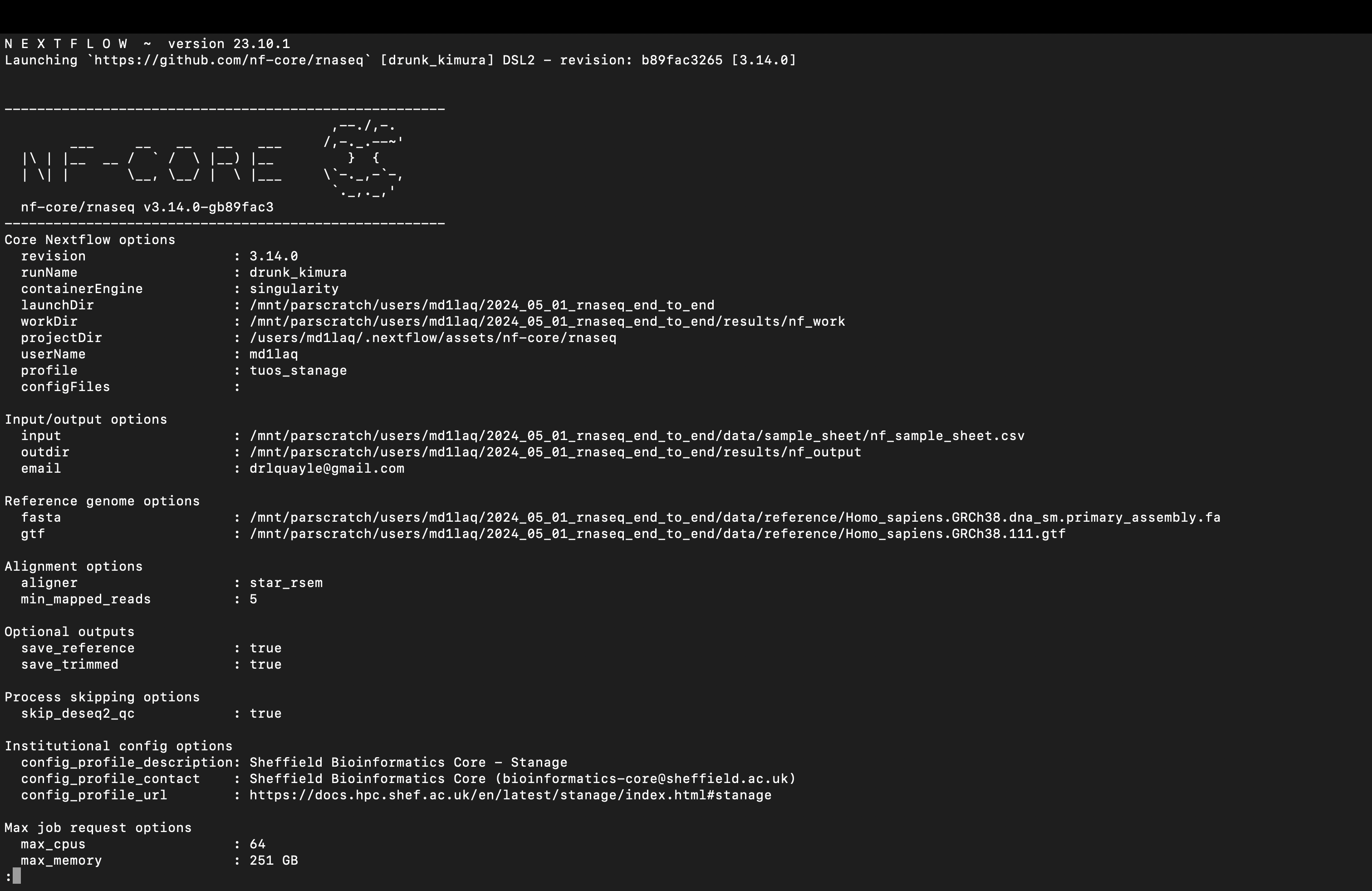
To get to the bottom of the document you can press shift + G to see the current processes in the pipeline being executed and Q to quit.
Once you’re happy that the pipeline is running, it’s time for a brew ☕ as it will take a couple of hours or so to run on a decent system (and longer on a less beefy HPC). It took 2h 36m 6s to run for me.
Download Results
Once the pipeline has finished running, we need to get hold of the results files that we need, but first you might want to setup the full local project directory tree on the machine that you’ll be analysing these processed data on using the one-line command shown below:
# make the project directory hierarchy
mkdir -p ./yyyy_mm_dd_rnaseq_end_to_end/{data/{processed,raw,reference,sample_sheet},docs,results/{figures,reports,tables},src/{nf_config,nf_params,r,shell}}
The most important results to transfer to a local machine are the pipeline execution report directory pipeline_info, the MultiQC report directory multiqc directory and the ready-made gene-level and transcript-level expression counts matrices inside the star_rsem directory, all four of which are TSV files beginning “rsem.merged.”. I also recommend spending some time downloading your source code and sample sheets, and making sure that your raw data are backed up e.g., on a cloud or data storage server. The project directory tree we just setup has directories to accomodate all the files that you might want to include in a self-contained project - use your judgement. A word of warning here: don’t just download the entire project directory from the HPC, it has some huge files (most of which you won’t need) and will be in excess of 200GB!
This is how your local project directory tree might look when you’re done:
/path/to/project/yyyy_mm_dd_rnaseq_end_to_end
|-- data
|   |-- processed
|   |   `-- star_rsem
|   |-- raw
|   |-- reference
|   `-- sample_sheet
|-- docs
|-- results
|   |-- figures
|   |-- reports
|   |   |-- multiqc
|   |   `-- pipeline_info
|   `-- tables
`-- src
    |-- nf_params
    |-- r
    `-- shell
To actually get the files or folders you need, different HPCs might have different recommended connection protocols e.g., scp, sftp, sshfs and others. Best to check your HPC documents or contact your system admin if you are unsure about how to transfer files to/from your HPC system. I usually just run a few scp request in my local terminal with the general structure shown below, making them recursive with the -r flag if I want a full directory as opposed to a single file:
scp -r $USER@$CLUSTER_NAME.institution.ac.uk:/path/to/project/yyyy_mm_dd_rnaseq_end_to_end /path/to/local/downloads
The reason I usually download and spend some time with the pipeline execution report is that it will allow you to finetune resource allocation for a similar pipeline run in future. The MultiQC report is not only critical for quality control but it also tells you about the pipeline run and tool versions you used when you come to write-up your results. A full rundown of QC is outside the scope of what I want to cover here. Phil Ewels, author of MultiQC and a lead figure in the nf-core project, has luckily already made a great introductory video on using MultiQC reports, so check that out if you are not sure what a MultiQC report is or how to get started with it.
Summary
That’s it! That’s all there is to analysing raw bulk RNA-Seq data and getting the files needed to progress the analysis of your experimental data set. Well, it’s a nice simple starter example at least.
Next time we will look at how to start analysing these data downstream in R, focussing on how to import them into your R environment, exploratory analysis of count data, normalisation strategies, quality assessment, and identification of outlier or mixed-up samples, batch effects and how to correct for these.
See you next time.
Thanks for reading. I hope you enjoyed the article and that it helps you to get a job done more quickly or inspires you to further your data science journey. Please do let me know if there’s anything you want me to cover in future posts.
If this tutorials has helped you, consider supporting the blog on Ko-fi!
Happy Data Analysis!
Disclaimer: All views expressed on this site are exclusively my own and do not represent the opinions of any entity whatsoever with which I have been, am now or will be affiliated.