Overview()
In the first part and second part of this series, I have been showing off some tips and tricks from the big bag of tricks that is the tidyverse.
This post will round out this mini-series and my current must-show list by demonstrating some intermediate-level essential tidyverse functions that massively speedup data wrangling when used properly, including a couple of widely neglected but super handy table joins.
TL;DW
In this tutorial, I use the volcano eruptions data set taken from the TidyTuesday project and cover how to wrangle data with the pivot_longer() and pivot_wider() functions from tidyr, and the family of join functions from dplyr; functions which every aspiring data scientist working in R should know and understand.
Tutorial Code
The first code block will load the packages required for the tutorial and setup a very modestly customised version of the theme_light() plotting theme that comes with ggplot2. This is just an optional extra based entirely on my personal preference for font size and element spacing.
# load libraries
library("tidyverse")

# custom plot theme
theme_custom <- function() {
  theme_light() +
    theme(
      axis.text = element_text(size = 10),
      axis.title.x = element_text(size = 12, margin = margin(t = 15)),
      axis.title.y = element_text(size = 12, margin = margin(r = 15)),
      panel.grid.minor = element_blank(),
      plot.margin = margin(1, 1, 1, 1, unit = "cm"),
      plot.title = element_text(size = 14, face = "bold", margin = margin(b = 10))
    )
}

# set plot theme
theme_set(theme_custom())
The data set used in this tutorial is the same volcano eruptions data set that was used in the previous two posts in this series. It was originally posted on the 12th of May 2020 as part of the weekly TidyTuesday project run by the R for Data Science Online Learning Community.
Only two of the five data tables from the full data set will be used here; these jointly give detailed information about global volcanoes and their location, geology, and eruptions events over time.
# load data
volcanoes <- read_csv("https://raw.githubusercontent.com/rfordatascience/tidytuesday/master/data/2020/2020-05-12/volcano.csv")
eruptions <- read_csv("https://raw.githubusercontent.com/rfordatascience/tidytuesday/master/data/2020/2020-05-12/eruptions.csv")
In the previous posts, we created a modestly cleaned version of the volcanoes table, so let’s reproduce that version of the data set so it can be used here.
# clean the 'primary_volcano_type' variable
volcanoes_cln <-
  volcanoes %>%
  mutate(
    primary_volcano_type = primary_volcano_type %>%
      str_remove("\\(.+\\)|\\?") %>%
      str_to_title()
  )
Now that we are all setup we can get on with the rest of the tutorial.
1. pivot_longer and pivot_wider
The most fundamental functions in the tidyverse for changing the shape of data are pivot_longer() and pivot_wider() from tidyr. The former lengthens data, decreasing the number of columns and increasing the number of rows, while the latter does the opposite.
In the data subset output from the chunk below, the population count at specified distances from each volcano is given across the 4 columns beginning with “population”.
volcanoes_cln %>%
  select(
    volcano_name,
    primary_volcano_type,
    population_within_5_km:last_col()
  )
# A tibble: 958 × 6
   volcano_name    primary_volcano_type population_within_5_km population_within_10_km population_within_30_km population_within_100_km
   <chr>           <chr>                                 <dbl>                   <dbl>                   <dbl>                    <dbl>
 1 Abu             Shield                                 3597                    9594                  117805                  4071152
 2 Acamarachi      Stratovolcano                             0                       7                     294                     9092
 3 Acatenango      Stratovolcano                          4329                   60730                 1042836                  7634778
 4 Acigol-Nevsehir Caldera                              127863                  127863                  218469                  2253483
 5 Adams           Stratovolcano                             0                      70                    4019                   393303
 6 Adatarayama     Stratovolcano                           428                    3936                  717078                  5024654
 7 Adwa            Stratovolcano                           101                     485                   18645                  1242922
 8 Afdera          Stratovolcano                            51                    6042                    8611                   161009
 9 Agrigan         Stratovolcano                             0                       0                       0                        0
10 Agua            Stratovolcano                          9890                  114404                 2530449                  7441660
# ℹ 948 more rows
# ℹ Use `print(n = ...)` to see more rows
The distance to the volcano and the population pertaining to each radius are essentially separate variables, so the pivot_longer() function can be used to reformat the data accordingly.
# pivot the data to long format
volcanoes_long <-
  volcanoes_cln %>%
  select(volcano_name, primary_volcano_type, population_within_5_km:last_col()) %>%
  pivot_longer(cols = starts_with("population"), names_to = "km_from_volcano", values_to = "population")

# print output
print(volcanoes_long)
# A tibble: 3,832 × 4
   volcano_name primary_volcano_type km_from_volcano          population
   <chr>        <chr>                <chr>                         <dbl>
 1 Abu          Shield               population_within_5_km         3597
 2 Abu          Shield               population_within_10_km        9594
 3 Abu          Shield               population_within_30_km      117805
 4 Abu          Shield               population_within_100_km    4071152
 5 Acamarachi   Stratovolcano        population_within_5_km            0
 6 Acamarachi   Stratovolcano        population_within_10_km           7
 7 Acamarachi   Stratovolcano        population_within_30_km         294
 8 Acamarachi   Stratovolcano        population_within_100_km       9092
 9 Acatenango   Stratovolcano        population_within_5_km         4329
10 Acatenango   Stratovolcano        population_within_10_km       60730
# ℹ 3,822 more rows
# ℹ Use `print(n = ...)` to see more rows
Using the pivot_longer() function, the numeric variables beginning with the string “population” in the input data frame have been converted into a new pair of variables; km_from_volcano contains the original column names and population is a new numeric variable containing their respective values.
As the newly created km_from_volcano variable only really needs to indicate the number of kilometres, a mutate() call can be added to this chunk in order clean and recode it as either an integer or an ordered categorical variable. In this case, I have chosen the latter and used the fct_inorder() function to do so is it will both coerce the variable to a factor and ensure the levels are in alphanumeric order; another handy function from forcats worth knowing about.
# pivot the data to long format
volcanoes_long <-
  volcanoes_cln %>%
  select(volcano_name, primary_volcano_type, population_within_5_km:last_col()) %>%
  pivot_longer(cols = starts_with("population"), names_to = "km_from_volcano", values_to = "population") %>%
  mutate(
    km_from_volcano = km_from_volcano %>%
      str_remove_all("population_within_|_km") %>%
      fct_inorder()
  )

# print output
print(volcanoes_long)
# A tibble: 3,832 × 4
   volcano_name primary_volcano_type km_from_volcano population
   <chr>        <chr>                <fct>                <dbl>
 1 Abu          Shield               5                     3597
 2 Abu          Shield               10                    9594
 3 Abu          Shield               30                  117805
 4 Abu          Shield               100                4071152
 5 Acamarachi   Stratovolcano        5                        0
 6 Acamarachi   Stratovolcano        10                       7
 7 Acamarachi   Stratovolcano        30                     294
 8 Acamarachi   Stratovolcano        100                   9092
 9 Acatenango   Stratovolcano        5                     4329
10 Acatenango   Stratovolcano        10                   60730
# ℹ 3,822 more rows
# ℹ Use `print(n = ...)` to see more rows
Where previously the population living within 5, 10, 30 and 100 kilometres would have been read across a single row for a specific named volcano, those data are now read down the rows and the volcano_name and primary_volcano_type entries repeated.
This data set is now be in the correct format for working with many of the functions from the tidyverse which use this so called “tidy data” format, where each variable must have its own column, each observation must have its own row and each value must have its own cell.
Now that the data in this format, filtering, grouping, and summarising the population data by volcano type and distance becomes possible. As an example, we could now easily make a plot of the number of people globally that live within 5, 10 and 30 kilometres of each type of volcano using tidyverse functions encountered previously in this series.
volcanoes_long %>%
  filter(km_from_volcano != 100) %>%
  count(primary_volcano_type, km_from_volcano, wt = population, name = "population") %>%

  ggplot(aes(x = km_from_volcano, y = population)) +
  geom_col() +
  scale_y_continuous(labels = scales::label_comma()) +
  facet_wrap(vars(primary_volcano_type), nrow = 4, scales = "free_y")
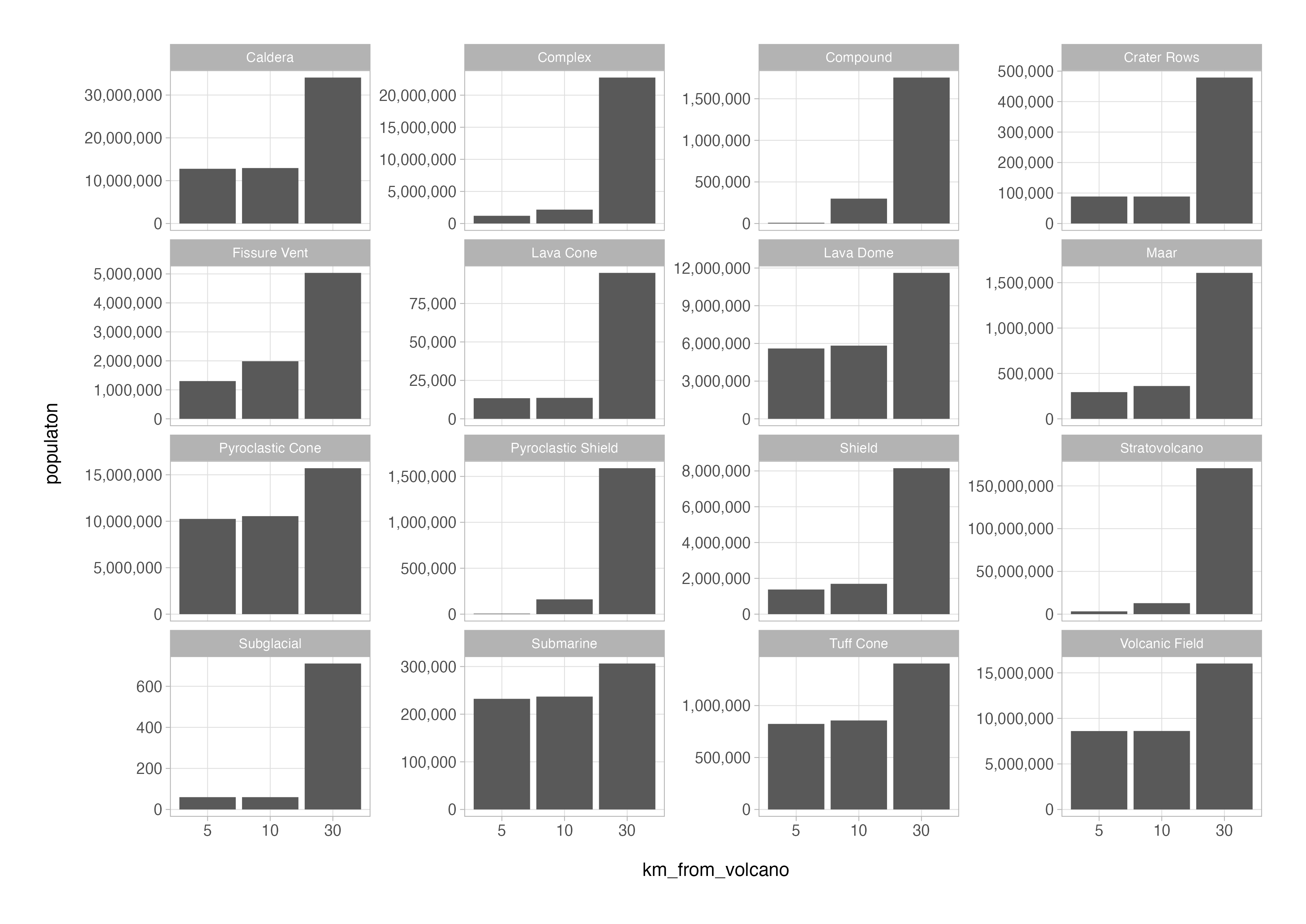
Now imagine that we wanted to create a table of the summarised data that we just plotted. The output of the count() call in the code chunk above still has the data in the long format with 48 rows with 3 columns.
volcanoes_long %>%
  filter(km_from_volcano != 100) %>%
  count(primary_volcano_type, km_from_volcano, wt = population, name = "population")
# A tibble: 48 × 3
   primary_volcano_type km_from_volcano population
   <chr>                <fct>                <dbl>
 1 Caldera              5                 12780739
 2 Caldera              10                12952021
 3 Caldera              30                34084720
 4 Complex              5                  1202049
 5 Complex              10                 2163137
 6 Complex              30                22744336
 7 Compound             5                     8962
 8 Compound             10                  299269
 9 Compound             30                 1754849
10 Crater Rows          5                    88566
# ℹ 38 more rows
# ℹ Use `print(n = ...)` to see more rows
In instances such as this, the pivot_wider() function can be used to decrease the number of rows and increase the number of columns by specifying the variables that the new column names and respective values will be taken from.
volcanoes_long %>%
  filter(km_from_volcano != 100) %>%
  count(primary_volcano_type, km_from_volcano, wt = population, name = "population") %>%
  pivot_wider(names_from = km_from_volcano, values_from = population, names_glue = "population_within_{km_from_volcano}_km")
# A tibble: 16 × 4
   primary_volcano_type population_within_5_km population_within_10_km population_within_30_km
   <chr>                                 <dbl>                   <dbl>                   <dbl>
 1 Caldera                            12780739                12952021                34084720
 2 Complex                             1202049                 2163137                22744336
 3 Compound                               8962                  299269                 1754849
 4 Crater Rows                           88566                   88566                  478837
 5 Fissure Vent                        1302684                 1986316                 5035797
 6 Lava Cone                             13413                   13623                   94911
 7 Lava Dome                           5598407                 5825023                11614460
 8 Maar                                 294252                  361538                 1608051
 9 Pyroclastic Cone                   10253577                10550737                15711417
10 Pyroclastic Shield                     5803                  161076                 1589513
11 Shield                              1375798                 1694992                 8152728
12 Stratovolcano                       3261340                12838863               170668994
13 Subglacial                               60                      60                     711
14 Submarine                            232263                  236950                  306359
15 Tuff Cone                            823520                  856631                 1404735
16 Volcanic Field                      8608891                 8617801                16024073
The non-mandatory names_glue argument is used here to create syntactically correct names for the newly created columns by adding a string either side of the number taken from the km_from_volcano variable in the input data frame. The names_prefix argument could be used instead to similar effect.
That’s all there is to the fundamentals of pivoting data in the tidyverse.
2. mutating joins
The very first thing to do before looking at how joins work is to pare down the variables in our data tables for clarity.
# reduced version of the volcanoes data frame
volcanoes_sm <-
  volcanoes_cln %>%
  select(
    volcano_number:primary_volcano_type,
    country,
    latitude:tectonic_settings,
    major_rock_1
  )

# reduced version of the eruptions data frame
eruptions_sm <-
  eruptions %>%
  select(
    volcano_number,
    eruption_number:eruption_category,
    vei:start_day,
    end_year:end_day
  )
The trick to understanding joins of any kind is to understand the concept of keys; a key is a variable (or set of variables) which has values that uniquely identify each observation in a table.
In this case, the volcano number is the key that will be used to join the volcanoes_sm and eruptions_sm tables as these meet the above definition; there are duplicate entries in the volcano_name variables.
Just like the mutate() function can be used to add new variables to a data frame, mutating joins are those which add columns to a specified data frame from another.
Mutating joins can be split into inner and outer joins.
An inner_join() adds variables from the second table to the first but keeps only the observations (or rows) where the keys from the first table are matched in the second table.
The most basic use of all the join functions is possible when we know that the keys in each table are identical and have the same variable name; in these instances, we only have to specify x and y arguments i.e., the two tables to join. Although this is possible, I would generally recommend being explicit about which variable(s) are being used as the key.
# basic use
volcanoes_sm %>%
  inner_join(eruptions_sm)

# explicitly specify the key variable(s) to join by
volcanoes_sm %>%
  inner_join(eruptions_sm, by = "volcano_number")
# A tibble: 9,559 × 18
   volcano_number volcano_name    primary_volcano_type country latitude longitude elevation tectonic_settings major_rock_1 eruption_number
            <dbl> <chr>           <chr>                <chr>      <dbl>     <dbl>     <dbl> <chr>             <chr>                  <dbl>
 1         283001 Abu             Shield               Japan       34.5     132.        641 Subduction zone … Andesite / …           17369
 2         342080 Acatenango      Stratovolcano        Guatem…     14.5     -90.9      3976 Subduction zone … Andesite / …           10655
 3         342080 Acatenango      Stratovolcano        Guatem…     14.5     -90.9      3976 Subduction zone … Andesite / …           10654
 4         342080 Acatenango      Stratovolcano        Guatem…     14.5     -90.9      3976 Subduction zone … Andesite / …           10653
 5         342080 Acatenango      Stratovolcano        Guatem…     14.5     -90.9      3976 Subduction zone … Andesite / …           10652
 6         342080 Acatenango      Stratovolcano        Guatem…     14.5     -90.9      3976 Subduction zone … Andesite / …           10651
 7         342080 Acatenango      Stratovolcano        Guatem…     14.5     -90.9      3976 Subduction zone … Andesite / …           10650
 8         342080 Acatenango      Stratovolcano        Guatem…     14.5     -90.9      3976 Subduction zone … Andesite / …           10649
 9         342080 Acatenango      Stratovolcano        Guatem…     14.5     -90.9      3976 Subduction zone … Andesite / …           10648
10         213004 Acigol-Nevsehir Caldera              Turkey      38.5      34.6      1683 Intraplate / Con… Rhyolite               13904
# ℹ 9,549 more rows
# ℹ 8 more variables: eruption_category <chr>, vei <dbl>, start_year <dbl>, start_month <dbl>, start_day <dbl>, end_year <dbl>,
#   end_month <dbl>, end_day <dbl>
# ℹ Use `print(n = ...)` to see more rows
In either case, the volcanoes_sm has been lengthened to include the information for the recorded eruptions for each of the volcanoes present in the eruptions_sm data set.
If the key variable(s) contain the same information but are named differently, the equivalent variables on which to join can be specified; several methods are detailed in the help documentation for the mutating joins (help("joins") or ?dplyr::'mutate-joins') but a named character vector is the most common.
# example code - not run
volcanoes_sm %>%
  inner_join(eruptions_sm, by = c("volcano_number" = "volcano_id"))
Along with inner_join() there are three more mutating joins which are collectively called outer joins all with similar syntax:
left_join()right_join()full_join()
A left_join() keeps all information in the first table and adds on information from the second where there is a matching key. Logically this means that you get the inner_join() plus you retain the rows of the first table where there was no matching key in the second table and the respective variables from the second table will be populated with NA values.
volcanoes_sm %>%
  left_join(eruptions_sm, by = "volcano_number")
# A tibble: 9,828 × 18
   volcano_number volcano_name primary_volcano_type country   latitude longitude elevation tectonic_settings  major_rock_1 eruption_number
            <dbl> <chr>        <chr>                <chr>        <dbl>     <dbl>     <dbl> <chr>              <chr>                  <dbl>
 1         283001 Abu          Shield               Japan         34.5     132.        641 Subduction zone /… Andesite / …           17369
 2         355096 Acamarachi   Stratovolcano        Chile        -23.3     -67.6      6023 Subduction zone /… Dacite                    NA
 3         342080 Acatenango   Stratovolcano        Guatemala     14.5     -90.9      3976 Subduction zone /… Andesite / …           10655
 4         342080 Acatenango   Stratovolcano        Guatemala     14.5     -90.9      3976 Subduction zone /… Andesite / …           10654
 5         342080 Acatenango   Stratovolcano        Guatemala     14.5     -90.9      3976 Subduction zone /… Andesite / …           10653
 6         342080 Acatenango   Stratovolcano        Guatemala     14.5     -90.9      3976 Subduction zone /… Andesite / …           10652
 7         342080 Acatenango   Stratovolcano        Guatemala     14.5     -90.9      3976 Subduction zone /… Andesite / …           10651
 8         342080 Acatenango   Stratovolcano        Guatemala     14.5     -90.9      3976 Subduction zone /… Andesite / …           10650
 9         342080 Acatenango   Stratovolcano        Guatemala     14.5     -90.9      3976 Subduction zone /… Andesite / …           10649
10         342080 Acatenango   Stratovolcano        Guatemala     14.5     -90.9      3976 Subduction zone /… Andesite / …           10648
# ℹ 9,818 more rows
# ℹ 8 more variables: eruption_category <chr>, vei <dbl>, start_year <dbl>, start_month <dbl>, start_day <dbl>, end_year <dbl>,
#   end_month <dbl>, end_day <dbl>
# ℹ Use `print(n = ...)` to see more rows
As predicted, this joined data frame has 9828 rows; 9559 rows of the inner join plus the 269 rows from the volcanoes_sm tables where there is no matching volcano number in the eruptions table.
A right_join() looks similar to a left join but it keeps all the information in the second table passed to the join rather than the first.
volcanoes_sm %>%
  right_join(eruptions_sm, by = "volcano_number")
# A tibble: 11,178 × 18
   volcano_number volcano_name    primary_volcano_type country latitude longitude elevation tectonic_settings major_rock_1 eruption_number
            <dbl> <chr>           <chr>                <chr>      <dbl>     <dbl>     <dbl> <chr>             <chr>                  <dbl>
 1         283001 Abu             Shield               Japan       34.5     132.        641 Subduction zone … Andesite / …           17369
 2         342080 Acatenango      Stratovolcano        Guatem…     14.5     -90.9      3976 Subduction zone … Andesite / …           10655
 3         342080 Acatenango      Stratovolcano        Guatem…     14.5     -90.9      3976 Subduction zone … Andesite / …           10654
 4         342080 Acatenango      Stratovolcano        Guatem…     14.5     -90.9      3976 Subduction zone … Andesite / …           10653
 5         342080 Acatenango      Stratovolcano        Guatem…     14.5     -90.9      3976 Subduction zone … Andesite / …           10652
 6         342080 Acatenango      Stratovolcano        Guatem…     14.5     -90.9      3976 Subduction zone … Andesite / …           10651
 7         342080 Acatenango      Stratovolcano        Guatem…     14.5     -90.9      3976 Subduction zone … Andesite / …           10650
 8         342080 Acatenango      Stratovolcano        Guatem…     14.5     -90.9      3976 Subduction zone … Andesite / …           10649
 9         342080 Acatenango      Stratovolcano        Guatem…     14.5     -90.9      3976 Subduction zone … Andesite / …           10648
10         213004 Acigol-Nevsehir Caldera              Turkey      38.5      34.6      1683 Intraplate / Con… Rhyolite               13904
# ℹ 11,168 more rows
# ℹ 8 more variables: eruption_category <chr>, vei <dbl>, start_year <dbl>, start_month <dbl>, start_day <dbl>, end_year <dbl>,
#   end_month <dbl>, end_day <dbl>
# ℹ Use `print(n = ...)` to see more rows
In this case all 11178 rows of the eruptions data are preserved but information will only be added from volcanoes_sm for the 689 volcanoes where there is a matching key in both tables; 242 volcanoes have multiple recorded eruptions in eruptions_sm but are absent from volcanoes_sm.
All of his means that we get the 9559 rows from the inner_join(), plus 1619 rows that exist in the eruptions data where there will be missing data for the variables in volcanoes_sm.
Right joins can be tricky for people, so I have included some code here enabling you to sanity check how I arrived at these numbers.
# entries where keys match
volcanoes_sm %>%
  right_join(eruptions_sm, by = "volcano_number") %>%
  filter(!is.na(primary_volcano_type)) %>% # this gives us an inner join
  nrow()

# entries where keys are absent in x
volcanoes_sm %>%
  right_join(eruptions_sm, by = "volcano_number") %>%
  filter(is.na(primary_volcano_type)) %>%
  nrow()

# volcanoes present in y but not x and number of observations (unique eruptions) for each
volcanoes_sm %>%
  right_join(eruptions_sm, by = "volcano_number") %>%
  filter(is.na(primary_volcano_type)) %>%
  count(volcano_number, sort = TRUE)
Mastering these joins and thereby the essentials of working with relational data in R is an essential skill.
3. filtering joins
The second major group of joins for working with relational data are the filtering joins. In dplyr the functions available for filtering joins are semi_join() and anti_join().
The call to both functions look almost identical to the other joins we have seen so far but their return values is what differs; they do not add any data but instead you get a reduced version of the table passed in as the x argument.
The semi_join() returns the rows from the first table passed to the join where there are matching keys in the second table.
volcanoes_sm %>%
  semi_join(eruptions_sm, by = "volcano_number")
# A tibble: 689 × 9
   volcano_number volcano_name    primary_volcano_type country       latitude longitude elevation tectonic_settings           major_rock_1
            <dbl> <chr>           <chr>                <chr>            <dbl>     <dbl>     <dbl> <chr>                       <chr>
 1         283001 Abu             Shield               Japan             34.5     132.        641 Subduction zone / Continen… Andesite / …
 2         342080 Acatenango      Stratovolcano        Guatemala         14.5     -90.9      3976 Subduction zone / Continen… Andesite / …
 3         213004 Acigol-Nevsehir Caldera              Turkey            38.5      34.6      1683 Intraplate / Continental c… Rhyolite
 4         321040 Adams           Stratovolcano        United States     46.2    -121.       3742 Subduction zone / Continen… Andesite / …
 5         283170 Adatarayama     Stratovolcano        Japan             37.6     140.       1728 Subduction zone / Continen… Andesite / …
 6         221170 Adwa            Stratovolcano        Ethiopia          10.1      40.8      1733 Rift zone / Intermediate c… Rhyolite
 7         284160 Agrigan         Stratovolcano        United States     18.8     146.        965 Subduction zone / Crustal … Basalt / Pi…
 8         342100 Agua            Stratovolcano        Guatemala         14.5     -90.7      3760 Subduction zone / Continen… Andesite / …
 9         382090 Agua de Pau     Stratovolcano        Portugal          37.8     -25.5       947 Rift zone / Oceanic crust … Trachyte / …
10         358062 Aguilera        Stratovolcano        Chile            -50.3     -73.8      2546 Subduction zone / Continen… Dacite
# ℹ 679 more rows
# ℹ Use `print(n = ...)` to see more rows
An anti_join() gives the inverse result of the semi_join(), that is, it returns the rows from the first table passed to the join where there is NOT a match in the second table.
volcanoes_sm %>%
  anti_join(eruptions_sm, by = "volcano_number")
# A tibble: 269 × 9
   volcano_number volcano_name     primary_volcano_type country    latitude longitude elevation tectonic_settings             major_rock_1
            <dbl> <chr>            <chr>                <chr>         <dbl>     <dbl>     <dbl> <chr>                         <chr>
 1         355096 Acamarachi       Stratovolcano        Chile        -23.3      -67.6      6023 Subduction zone / Continenta… Dacite
 2         221110 Afdera           Stratovolcano        Ethiopia      13.1       40.9      1250 Rift zone / Intermediate cru… Rhyolite
 3         282022 Akusekijima      Stratovolcano        Japan         29.5      130.        555 Subduction zone / Oceanic cr… Andesite / …
 4         221090 Ale Bagu         Stratovolcano        Ethiopia      13.5       40.6       988 Rift zone / Intermediate cru… Basalt / Pi…
 5         221040 Alid             Stratovolcano        Eritrea       14.9       39.9       904 Rift zone / Intermediate cru… Rhyolite
 6         320020 Alligator Lake   Volcanic Field       Canada        60.4     -135.       2217 Intraplate / Continental cru… Basalt / Pi…
 7         268072 Amasing          Stratovolcano        Indonesia     -0.53     127.       1030 Subduction zone / Oceanic cr… Andesite / …
 8         233011 Ambre-Bobaomby   Volcanic Field       Madagascar   -12.6       49.2      1475 Intraplate / Continental cru… Basalt / Pi…
 9         234001 Amsterdam Island Stratovolcano        France       -37.8       77.5       881 Rift zone / Oceanic crust (<… Basalt / Pi…
10         300390 Anaun            Stratovolcano        Russia        56.3      159.       1828 Subduction zone / Continenta… Basalt / Pi…
# ℹ 259 more rows
# ℹ Use `print(n = ...)` to see more rows
In both cases, if you were more interested in the eruptions_sm data and finding out about the number of matches, or filtering to remove the data that was missing but without joining the tables up, then you would just reverse the order of the tables passed to the x and y arguments.
Summary()
That brings me to the end of this tutorial and this entire mini-series. That said, I really enjoy showing the handiest functions and nifty little ways of using them to fellow R users, so no doubt I will be back at some point with more tidyverse tips and tricks to elevate your R code.
In the meantime, I hope you enjoyed the video and the tutorial, please like, and subscribe to my YouTube channel if you want to keep up to date with my latest tutorial videos, and feel free to get in touch in the comments or via my website.
Catch you next time!
View Session Info
## ─ Session info ───────────────────────────────────────────────────────────────
## setting  value
## version  R version 4.2.1 (2022-06-23)
## os       macOS 14.0
## system   x86_64, darwin17.0
## ui       RStudio
## language (EN)
## collate  en_US.UTF-8
## ctype    en_US.UTF-8
## tz       Europe/London
## date     2023-12-06
## rstudio  2023.03.2+454 Cherry Blossom (desktop)
## pandoc   2.19.2 @ /Applications/RStudio.app/Contents/Resources/app/quarto/bin/tools/ (via rmarkdown)
## ─ Packages ───────────────────────────────────────────────────────────────────
## package     * version date (UTC) lib source
## bit           4.0.5   2022-11-15 [1] CRAN (R 4.2.0)
## bit64         4.0.5   2020-08-30 [1] CRAN (R 4.2.0)
## cli           3.6.1   2023-03-23 [1] CRAN (R 4.2.0)
## colorspace    2.1-0   2023-01-23 [1] CRAN (R 4.2.0)
## crayon        1.5.2   2022-09-29 [1] CRAN (R 4.2.0)
## curl          5.0.1   2023-06-07 [1] CRAN (R 4.2.0)
## digest        0.6.33  2023-07-07 [1] CRAN (R 4.2.1)
## dplyr       * 1.1.2   2023-04-20 [1] CRAN (R 4.2.1)
## evaluate      0.21    2023-05-05 [1] CRAN (R 4.2.0)
## fansi         1.0.4   2023-01-22 [1] CRAN (R 4.2.0)
## farver        2.1.1   2022-07-06 [1] CRAN (R 4.2.0)
## fastmap       1.1.1   2023-02-24 [1] CRAN (R 4.2.0)
## forcats     * 1.0.0   2023-01-29 [1] CRAN (R 4.2.0)
## generics      0.1.3   2022-07-05 [1] CRAN (R 4.2.0)
## ggplot2     * 3.4.2   2023-04-03 [1] CRAN (R 4.2.0)
## glue          1.6.2   2022-02-24 [1] CRAN (R 4.2.0)
## gtable        0.3.3   2023-03-21 [1] CRAN (R 4.2.0)
## hms           1.1.3   2023-03-21 [1] CRAN (R 4.2.0)
## htmltools     0.5.5   2023-03-23 [1] CRAN (R 4.2.0)
## knitr         1.43    2023-05-25 [1] CRAN (R 4.2.0)
## labeling      0.4.2   2020-10-20 [1] CRAN (R 4.2.0)
## lifecycle     1.0.3   2022-10-07 [1] CRAN (R 4.2.1)
## lubridate   * 1.9.2   2023-02-10 [1] CRAN (R 4.2.0)
## magrittr      2.0.3   2022-03-30 [1] CRAN (R 4.2.0)
## munsell       0.5.0   2018-06-12 [1] CRAN (R 4.2.0)
## pillar        1.9.0   2023-03-22 [1] CRAN (R 4.2.0)
## pkgconfig     2.0.3   2019-09-22 [1] CRAN (R 4.2.0)
## purrr       * 1.0.1   2023-01-10 [1] CRAN (R 4.2.0)
## R6            2.5.1   2021-08-19 [1] CRAN (R 4.2.0)
## readr       * 2.1.4   2023-02-10 [1] CRAN (R 4.2.0)
## rlang         1.1.1   2023-04-28 [1] CRAN (R 4.2.0)
## rmarkdown     2.23    2023-07-01 [1] CRAN (R 4.2.0)
## rstudioapi    0.15.0  2023-07-07 [1] CRAN (R 4.2.0)
## scales        1.2.1   2022-08-20 [1] CRAN (R 4.2.0)
## sessioninfo   1.2.2   2021-12-06 [1] CRAN (R 4.2.0)
## SnowballC     0.7.1   2023-04-25 [1] CRAN (R 4.2.0)
## stringi       1.7.12  2023-01-11 [1] CRAN (R 4.2.0)
## stringr     * 1.5.0   2022-12-02 [1] CRAN (R 4.2.0)
## tibble      * 3.2.1   2023-03-20 [1] CRAN (R 4.2.0)
## tidyr       * 1.3.0   2023-01-24 [1] CRAN (R 4.2.1)
## tidyselect    1.2.0   2022-10-10 [1] CRAN (R 4.2.0)
## tidyverse   * 2.0.0   2023-02-22 [1] CRAN (R 4.2.0)
## timechange    0.2.0   2023-01-11 [1] CRAN (R 4.2.0)
## tzdb          0.4.0   2023-05-12 [1] CRAN (R 4.2.0)
## utf8          1.2.3   2023-01-31 [1] CRAN (R 4.2.0)
## vctrs         0.6.3   2023-06-14 [1] CRAN (R 4.2.0)
## vroom         1.6.3   2023-04-28 [1] CRAN (R 4.2.0)
## withr         2.5.0   2022-03-03 [1] CRAN (R 4.2.0)
## xfun          0.39    2023-04-20 [1] CRAN (R 4.2.1)
## yaml          2.3.7   2023-01-23 [1] CRAN (R 4.2.0)
##
## [1] /Library/Frameworks/R.framework/Versions/4.2/Resources/library
##
## ──────────────────────────────────────────────────────────────────────────────
Thanks for reading. I hope you enjoyed the article and that it helps you to get a job done more quickly or inspires you to further your data science journey. Please do let me know if there’s anything you want me to cover in future posts.
If this tutorials has helped you, consider buying me a coffee on Ko-fi!
Happy Data Analysis!
Disclaimer: All views expressed on this site are exclusively my own and do not represent the opinions of any entity whatsoever with which I have been, am now or will be affiliated.