This Post is My Recital…
To paraphrase Run-D.M.C. “It’s not tricky to use R tricks, to use R tricks to get your kicks, not Tricky…Tr-tr-tr-tricky (Tricky) Trrrrrrrrrrricky”.
OK, that was terrible. The good news is that I am a lot better at R than I am at thinking up blog post introductions.
In the previous post, I started to showcase some neat tricks and lesser-known functions from the tidyverse that are easy to implement in your R workflows in order to streamline code and save time. This post is more of the same.
TL;DW
In this tutorial, I use the volcano eruptions data set taken from the TidyTuesday project and introduce some staple functions from the tidyverse and tidytext packages that are incredibly useful (and convenient) for the common tasks of working with and plotting categorical variables.
Tutorial Code
As usual, the first code block will load the packages required for the tutorial. It also includes some code to setup a very modestly customised version of the theme_light() plotting theme that comes with ggplot2. This is just an optional extra based entirely on my personal preference for font size and element spacing.
# load libraries
library("tidyverse")
library("tidytext")

# custom plot theme
theme_custom <- function() {
  theme_light() +
    theme(
      axis.text = element_text(size = 10),
      axis.title.x = element_text(size = 12, margin = margin(t = 15)),
      axis.title.y = element_text(size = 12, margin = margin(r = 15)),
      panel.grid.minor = element_blank(),
      plot.margin = margin(1, 1, 1, 1, unit = "cm"),
      plot.title = element_text(size = 14, face = "bold", margin = margin(b = 10))
    )
}

# set plot theme
theme_set(theme_custom())
The data set used in this tutorial is the same volcano eruptions data set that was used in the previous post. It was originally posted on the 12th of May 2020 as part of the weekly TidyTuesday project run by the R for Data Science Online Learning Community.
# load data
volcanoes <- read_csv("https://raw.githubusercontent.com/rfordatascience/tidytuesday/master/data/2020/2020-05-12/volcano.csv")
eruptions <- read_csv("https://raw.githubusercontent.com/rfordatascience/tidytuesday/master/data/2020/2020-05-12/eruptions.csv")
In the previous post, we created a cleaned version of the volcanoes table, so let’s reproduce that cleaned version so that we can use it in this tutorial.
# clean the 'primary_volcano_type' variable
volcanoes_cln <-
  volcanoes %>%
  mutate(
    primary_volcano_type = primary_volcano_type %>%
      str_remove("\\(.+\\)|\\?") %>%
      str_to_title()
  )
Now that we are all setup we can get on with the tutorial.
1. fct_lump
The fct_lump() series of functions from the forcats package are used for binning the less frequent levels in a categorical variable into a single level. The fct_lump_n() variation used below, which lumps all levels except for the n most frequent, is probably the most useful variant.
volcanoes_cln %>%
  count(
    volcano_type = fct_lump_n(primary_volcano_type, n = 2),
    name = "count",
    sort = TRUE
  )
# A tibble: 3 × 2
  primary_volcano_type count
  <fct>                <int>
1 Stratovolcano          461
2 Other                  379
3 Shield                 118
Here, the 16 original levels in the primary_volcano_type variable from the volcanoes_cln data frame are reduced to only the two largest groups and a third with all the other less frequently occurring levels combined. In this case, using fct_lump_n() inside the call to count() has enabled us to create and count the binned volcano_type variable on the fly, which we could have done prior to the call to count() inside mutate().
Refer to the help documents for this series of functions using help("fct_lump") or ?forcats::fct_lump to view the alternative versions that are available to lump infrequently occurring categories based on a minimum threshold or occurrence above a threshold proportion of the total.
2. bar charts
The usual way of visualising simple frequency counts for categorical variables is a bar chart. If the frequency counts are pre-computed (e.g., using count() function) then we must use the geom_col() geometry when plotting in ggplot2 rather than geom_bar() which only requires a single aesthetic mapping. I mention this as it trips new users up all the time!
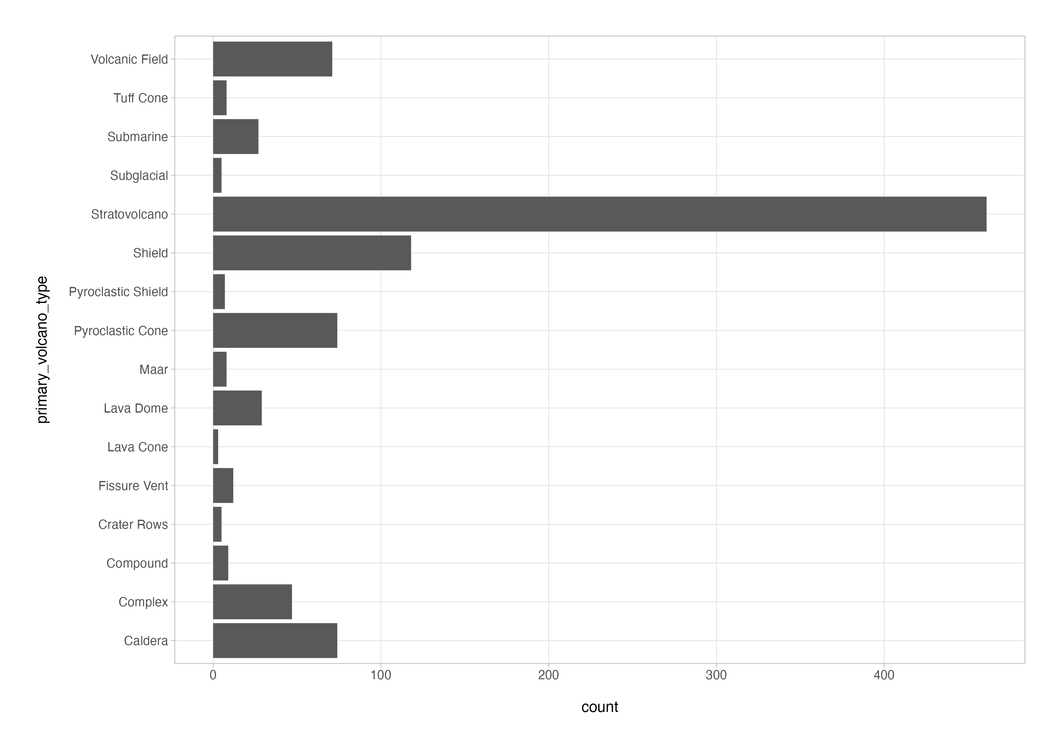
Possibly the most useful plot when conducting exploratory data analysis is variant on the simple bar chart in which the categorical variable is mapped to the y-axis and arranged in descending order of the magnitude of the frequency counts.
There are two options for making the basis for this plot that you will usually see in the wild:
# option 1 - use `coord_flip()`
volcanoes_cln %>%
  count(primary_volcano_type, name = "count", sort = TRUE) %>%

  ggplot(aes(x = primary_volcano_type, y = count)) +
  geom_col() +
  coord_flip()

# option 2 - reverse the variable-axis mapping
volcanoes_cln %>%
  count(primary_volcano_type, name = "count", sort = TRUE) %>%

  ggplot(aes(x = count, y = primary_volcano_type)) +
  geom_col()
The first option is vestigial and originates from the dark times when the second option was not possible in ggplot2. I personally prefer and use the latter option when making bar charts, but there are more specific instances where coord_flip() is the only viable means of achieving flipped axes, so a good one to know.
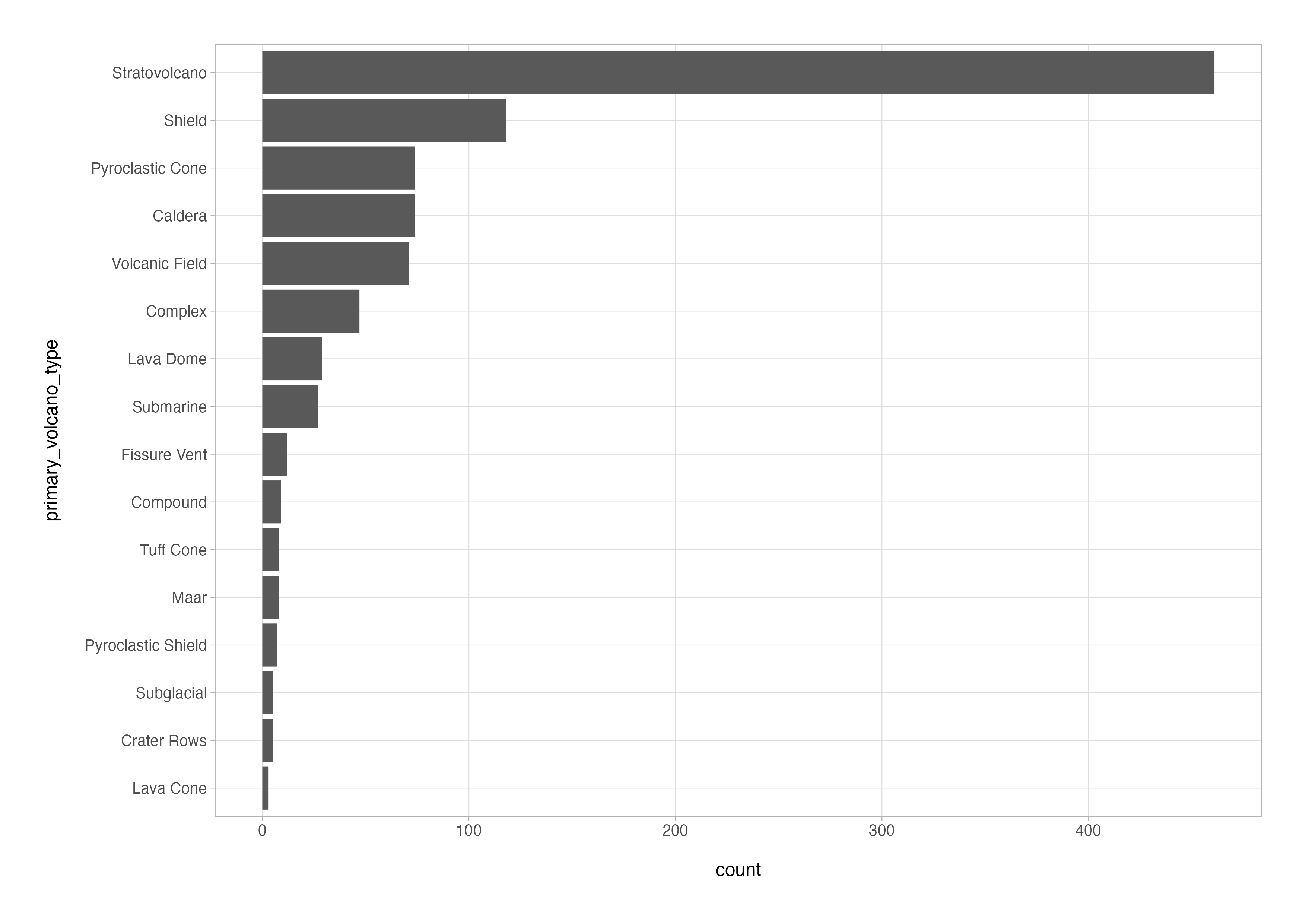
3. fct_reorder
The fct_reorder() function is required to arrange the bars on the previous plot in order of the magnitude of the frequency counts; this doesn’t happen despite the output of the count() function being sorted because the categorical variable is plotted as a factor in alphanumeric order by default.
You can do the factor reordering within the plotting code, saving you the mutate() call in the code below, but I prefer to keep my data wrangling and plotting code separate as much as possible.
volcanoes_cln %>%
  count(primary_volcano_type, name = "count", sort = TRUE) %>%
  mutate(primary_volcano_type = fct_reorder(primary_volcano_type, count)) %>%

  ggplot(aes(x = count, y = primary_volcano_type)) +
  geom_col()
There are many more modifications you could make to prettify this plot. If you want to learn more about how to use ggplot2, I wrote an introduction to ggplot2 series a little while ago which covers how to do just that.
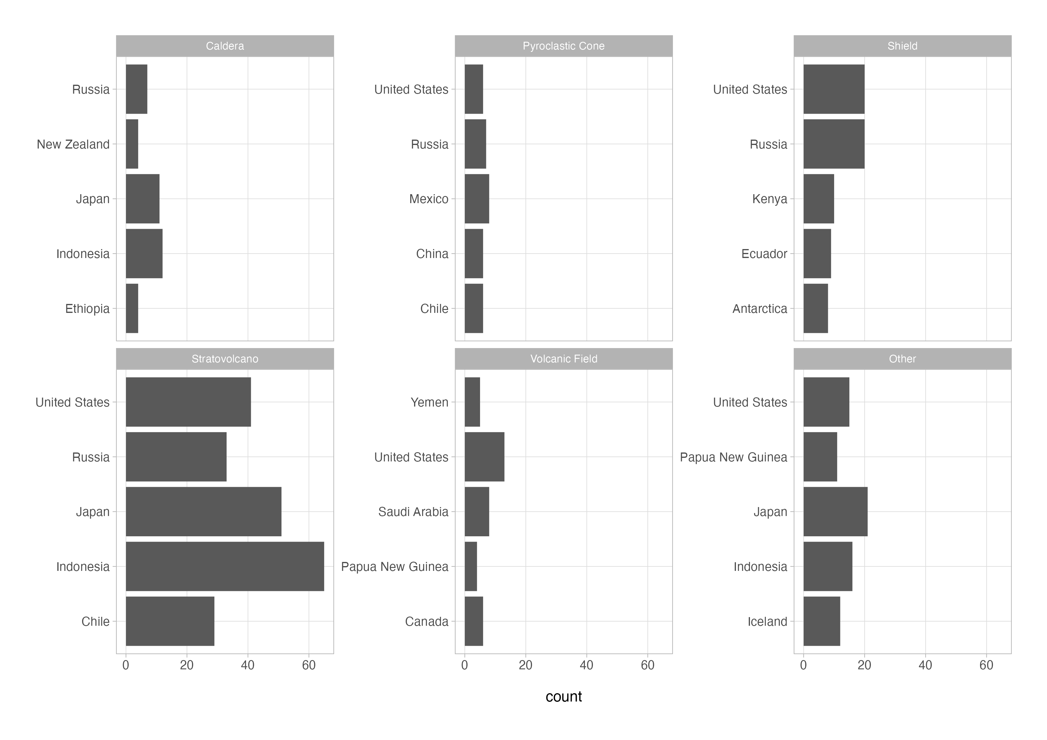
4. reordering inside facets
Reorder the bars on faceted plots isn’t something that is natively easy to do with just the core tidyverse. Luckily, the tidytext package that we loaded in the first code chunk contains a couple of functions for this purpose.
Below is some code which creates a basic faceted plot with unordered bars:
volcanoes_cln %>%
  count(country, primary_volcano_type = fct_lump(primary_volcano_type, n = 5), name = "count", sort = TRUE) %>%
  group_by(primary_volcano_type) %>%
  slice_max(n = 5, order_by = count, with_ties = FALSE) %>%
  ungroup() %>%

  ggplot(aes(x = count, y = country)) +
  geom_col() +
  facet_wrap(vars(primary_volcano_type), scales = "free_y") +
  labs(y = NULL)
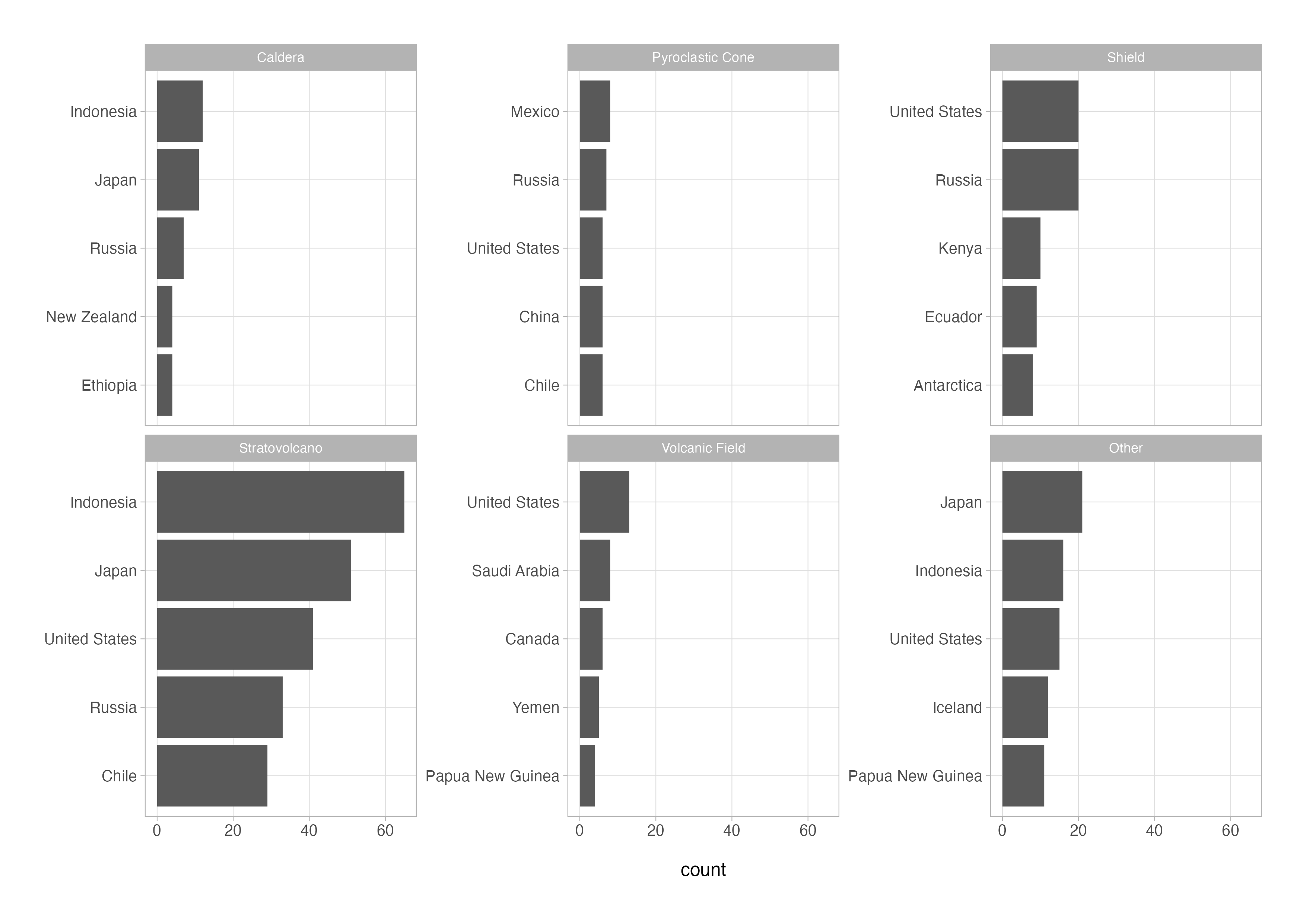
The same code is presented below with two additional lines of code highlighted that use the reorder_within() and scale_y_reordered() functions from tidytext in order to reorder the bars independently within each facet.
volcanoes_cln %>%
  count(country, primary_volcano_type = fct_lump_n(primary_volcano_type, n = 5), name = "count", sort = TRUE) %>%
  group_by(primary_volcano_type) %>%
  slice_max(n = 5, order_by = count, with_ties = FALSE) %>%
  ungroup() %>%

  # reorders the bars within facets
  mutate(country = reorder_within(country, count, primary_volcano_type)) %>%

  ggplot(aes(x = count, y = country)) +
  geom_col() +

  # removes the automatic y-axis labels
  scale_y_reordered() +

  facet_wrap(vars(primary_volcano_type), nrow = 2, scales = "free_y") +
  labs(y = NULL)
The tidytext package is not just equipped with nifty little functions like this but is the go-to for anyone using the R ecosystem for text analysis and natural language processing. Well worth a look.
Summary()
That brings me to the end of another set of tips and tricks. In the next post in this series, we will look at useful intermediate level functions for reshaping and joining tables of data.
In the meantime, I hope you enjoyed the video and the tutorial, please like, and subscribe to my YouTube channel if you want to keep up to date with my latest tutorial videos, and feel free to get in touch in the comments or via my website.
Catch you next time!
View Session Info
## ─ Session info ───────────────────────────────────────────────────────────────
## setting  value
## version  R version 4.2.1 (2022-06-23)
## os       macOS Ventura 13.4
## system   x86_64, darwin17.0
## ui       RStudio
## language (EN)
## collate  en_US.UTF-8
## ctype    en_US.UTF-8
## tz       Europe/London
## date     2023-09-13
## rstudio  2023.03.2+454 Cherry Blossom (desktop)
## pandoc   2.19.2 @ /Applications/RStudio.app/Contents/Resources/app/quarto/bin/tools/ (via rmarkdown)
## ─ Packages ───────────────────────────────────────────────────────────────────
## package     * version date (UTC) lib source
## bit           4.0.5   2022-11-15 [1] CRAN (R 4.2.0)
## bit64         4.0.5   2020-08-30 [1] CRAN (R 4.2.0)
## cli           3.6.1   2023-03-23 [1] CRAN (R 4.2.0)
## colorspace    2.1-0   2023-01-23 [1] CRAN (R 4.2.0)
## crayon        1.5.2   2022-09-29 [1] CRAN (R 4.2.0)
## curl          5.0.2   2023-08-14 [1] CRAN (R 4.2.0)
## digest        0.6.33  2023-07-07 [1] CRAN (R 4.2.1)
## dplyr       * 1.1.2   2023-04-20 [1] CRAN (R 4.2.1)
## evaluate      0.21    2023-05-05 [1] CRAN (R 4.2.0)
## fansi         1.0.4   2023-01-22 [1] CRAN (R 4.2.0)
## farver        2.1.1   2022-07-06 [1] CRAN (R 4.2.0)
## fastmap       1.1.1   2023-02-24 [1] CRAN (R 4.2.0)
## forcats     * 1.0.0   2023-01-29 [1] CRAN (R 4.2.0)
## generics      0.1.3   2022-07-05 [1] CRAN (R 4.2.0)
## ggplot2     * 3.4.3   2023-08-14 [1] CRAN (R 4.2.0)
## glue          1.6.2   2022-02-24 [1] CRAN (R 4.2.0)
## gtable        0.3.4   2023-08-21 [1] CRAN (R 4.2.0)
## hms           1.1.3   2023-03-21 [1] CRAN (R 4.2.0)
## htmltools     0.5.6   2023-08-10 [1] CRAN (R 4.2.0)
## janeaustenr   1.0.0   2022-08-26 [1] CRAN (R 4.2.0)
## knitr         1.43    2023-05-25 [1] CRAN (R 4.2.0)
## labeling      0.4.2   2020-10-20 [1] CRAN (R 4.2.0)
## lattice       0.21-8  2023-04-05 [1] CRAN (R 4.2.0)
## lifecycle     1.0.3   2022-10-07 [1] CRAN (R 4.2.1)
## lubridate   * 1.9.2   2023-02-10 [1] CRAN (R 4.2.0)
## magrittr      2.0.3   2022-03-30 [1] CRAN (R 4.2.0)
## Matrix        1.5-4.1 2023-05-18 [1] CRAN (R 4.2.0)
## munsell       0.5.0   2018-06-12 [1] CRAN (R 4.2.0)
## pillar        1.9.0   2023-03-22 [1] CRAN (R 4.2.0)
## pkgconfig     2.0.3   2019-09-22 [1] CRAN (R 4.2.0)
## purrr       * 1.0.2   2023-08-10 [1] CRAN (R 4.2.0)
## R6            2.5.1   2021-08-19 [1] CRAN (R 4.2.0)
## Rcpp          1.0.11  2023-07-06 [1] CRAN (R 4.2.1)
## readr       * 2.1.4   2023-02-10 [1] CRAN (R 4.2.0)
## rlang         1.1.1   2023-04-28 [1] CRAN (R 4.2.0)
## rmarkdown     2.24    2023-08-14 [1] CRAN (R 4.2.0)
## rstudioapi    0.15.0  2023-07-07 [1] CRAN (R 4.2.0)
## scales        1.2.1   2022-08-20 [1] CRAN (R 4.2.0)
## sessioninfo   1.2.2   2021-12-06 [1] CRAN (R 4.2.0)
## SnowballC     0.7.1   2023-04-25 [1] CRAN (R 4.2.0)
## stringi       1.7.12  2023-01-11 [1] CRAN (R 4.2.0)
## stringr     * 1.5.0   2022-12-02 [1] CRAN (R 4.2.0)
## tibble      * 3.2.1   2023-03-20 [1] CRAN (R 4.2.0)
## tidyr       * 1.3.0   2023-01-24 [1] CRAN (R 4.2.1)
## tidyselect    1.2.0   2022-10-10 [1] CRAN (R 4.2.0)
## tidytext    * 0.4.1   2023-01-07 [1] CRAN (R 4.2.0)
## tidyverse   * 2.0.0   2023-02-22 [1] CRAN (R 4.2.0)
## timechange    0.2.0   2023-01-11 [1] CRAN (R 4.2.0)
## tokenizers    0.3.0   2022-12-22 [1] CRAN (R 4.2.0)
## tzdb          0.4.0   2023-05-12 [1] CRAN (R 4.2.0)
## utf8          1.2.3   2023-01-31 [1] CRAN (R 4.2.0)
## vctrs         0.6.3   2023-06-14 [1] CRAN (R 4.2.0)
## vroom         1.6.3   2023-04-28 [1] CRAN (R 4.2.0)
## withr         2.5.0   2022-03-03 [1] CRAN (R 4.2.0)
## xfun          0.40    2023-08-09 [1] CRAN (R 4.2.0)
## yaml          2.3.7   2023-01-23 [1] CRAN (R 4.2.0)
##
## [1] /Library/Frameworks/R.framework/Versions/4.2/Resources/library
##
## ──────────────────────────────────────────────────────────────────────────────
Thanks for reading. I hope you enjoyed the article and that it helps you to get a job done more quickly or inspires you to further your data science journey. Please do let me know if there’s anything you want me to cover in future posts.
Happy Data Analysis!
Disclaimer: All views expressed on this site are exclusively my own and do not represent the opinions of any entity whatsoever with which I have been, am now or will be affiliated.