ggplot(recap)
In the first part of this introduction to ggplot2 series, we introduced the “Layered Grammar of Graphics” and how to create aesthetic mappings between variables in your data and plot scales. In part two we covered modifying aesthetics and attributes, as well as looking at rudimentary versions of common plot types.
 Source:
xkcd.com
Source:
xkcd.com
In this post, we are going to look at a framework for customising the non-data elements of your plots and learn an easy way to export high-quality graphics using ggplot2. Say goodbye to your days of making those horrible graphics rendered in Microsoft Office.
Setup
We will be working with the IMDb top-rated data set that we have been using throughout this mini-series; the data set can be downloaded from here if you don’t already have it. If you want to learn more about how these data were harvested, checkout my series on basic web scraping in R.
As in the previous post, you will need to have installed and loaded the dplyr and ggplot2 packages. If you do not have these installed, the most convenient way to get them is to install the packages that form the tidyverse by running install.packages("tidyverse") once before loading our dependencies for this tutorial:
# load packages
library("dplyr")
library("ggplot2")
We can use the load() function with the path to the Rds file in order to load in the data. I am going to load the data directly from my default downloads directory:
# load imdb top-rated data set
load(file = file.path("~", "Downloads", "imdb_top_rated_clean.rds"))
We will then need to quickly remove some rows with missing values in a couple of variables that I intentionally left in for a future data cleaning tutorial; removing these rows will help us focus on what’s going on in the plotting code and not get distracted by having to wrangle the data.
# remove missing observations from the data
imdb_data_clean <- imdb_data %>%
  filter(!is.na(gross_boxoffice) & !is.na(metascores))
One last thing I have chosen to do is change the default base theme used for plotting to theme_light(); this step is personal preference and entirely optional.
# update the default theme used for plotting to theme_light()
theme_set(theme_light())
Now, let’s make some more graphs.
The theme() Layer
The theme layer controls all the non-data ink on a plot; these are all the visual elements that are not actually formed by the data.
Visual elements can be classified as being either text, line, or rectangle. Each of these can be modified using a related function that begins with the common root element_ followed by either text, line, or rect, depending on which visual element it pertains to; the three key visual element functions are therefore element_text(), element_line() or element_rect().
Let’s start by generating a plot we saw last time so that we can customise it further throughout this tutorial to demonstrate common ggplot2 functions used in theming.
# define a reproducible jitter variable using position_jitter()
jitter <- position_jitter(
width = 0.1,
seed = 123
)
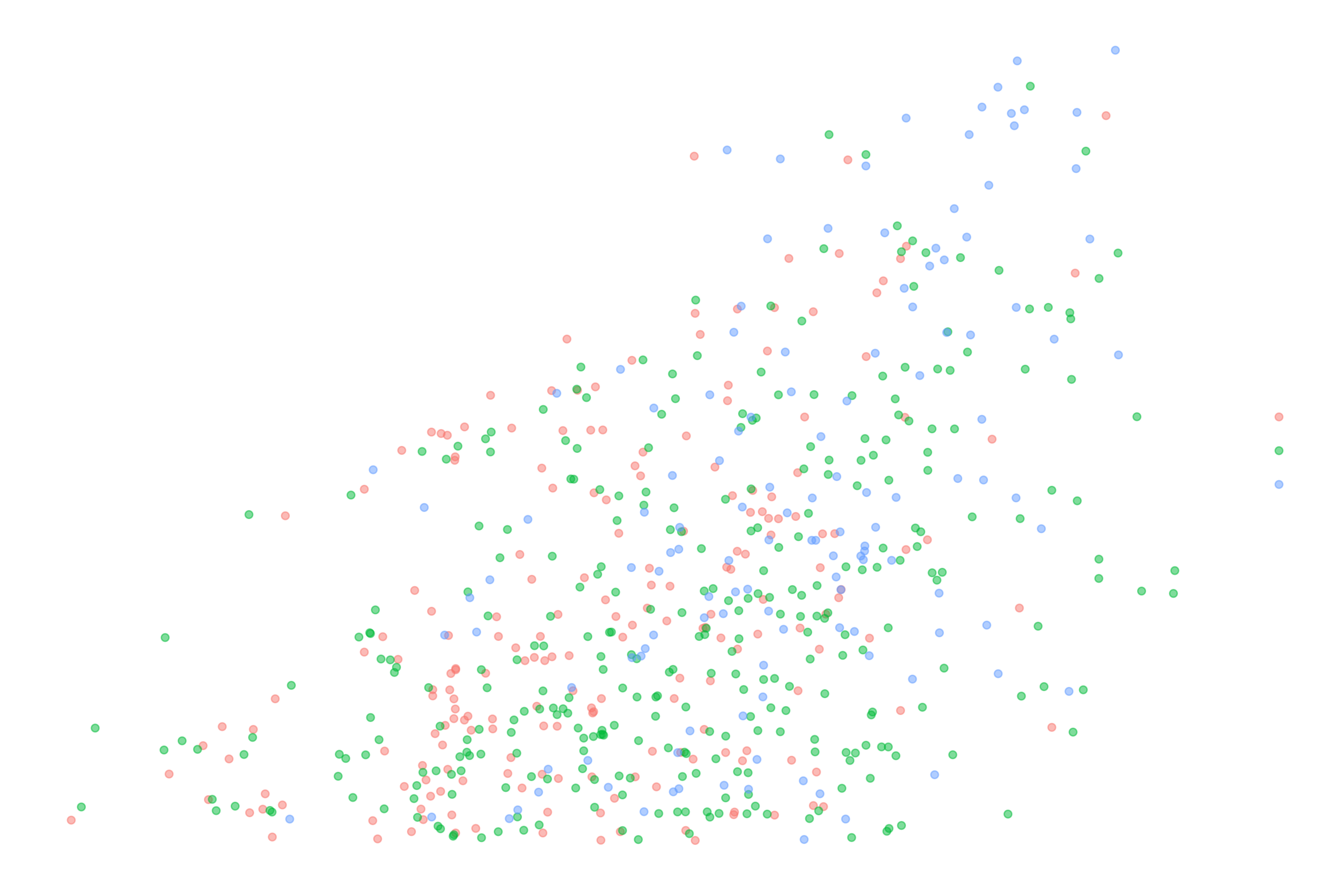
# base plot code
ggplot(imdb_data_clean, aes(x = imdb_rating, y = metascores, colour = genre)) +
geom_point(position = jitter, alpha = 0.5)
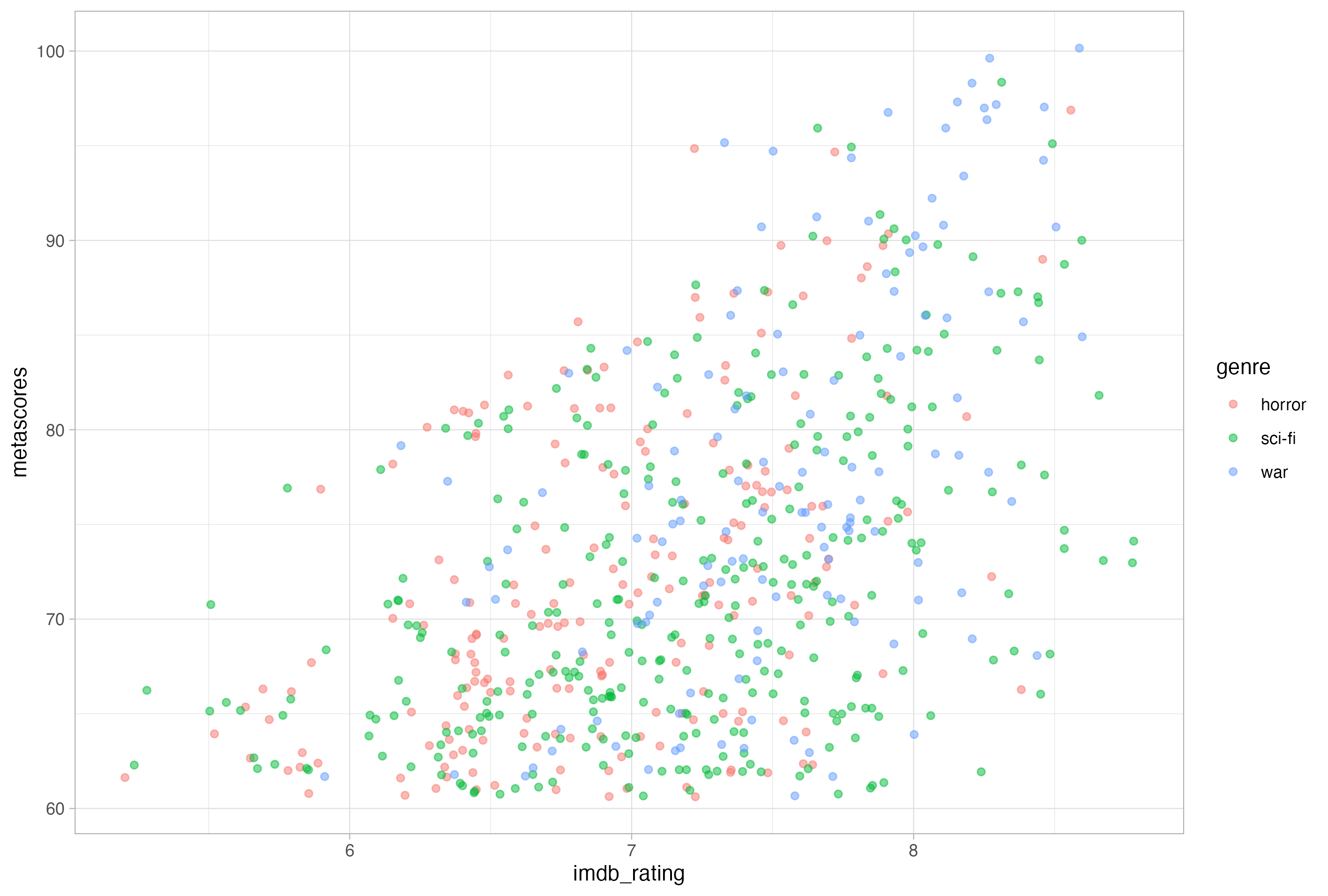
Considering the plot we have just produced, we can see that it is composed out of a combination of data and various non-data embellishments. For example, I have highlighted below all the text elements on our plot:
All non-data plot elements have corresponding arguments to the theme() function. Like all other layers in ggplot2, the theme layer is accessed by adding it to the plot with the + operator.
# not run
ggplot(imdb_data_clean, aes(x = imdb_rating, y = metascores)) +
  geom_point(aes(colour = genre), position = jitter, alpha = 0.5) +
  theme()
In order to modify an element within the theme layer, find the argument relating to the plot element that you wish to modify and call the appropriate element_ function inside the theme() layer in order specify what you want to change and how you would like to change it.
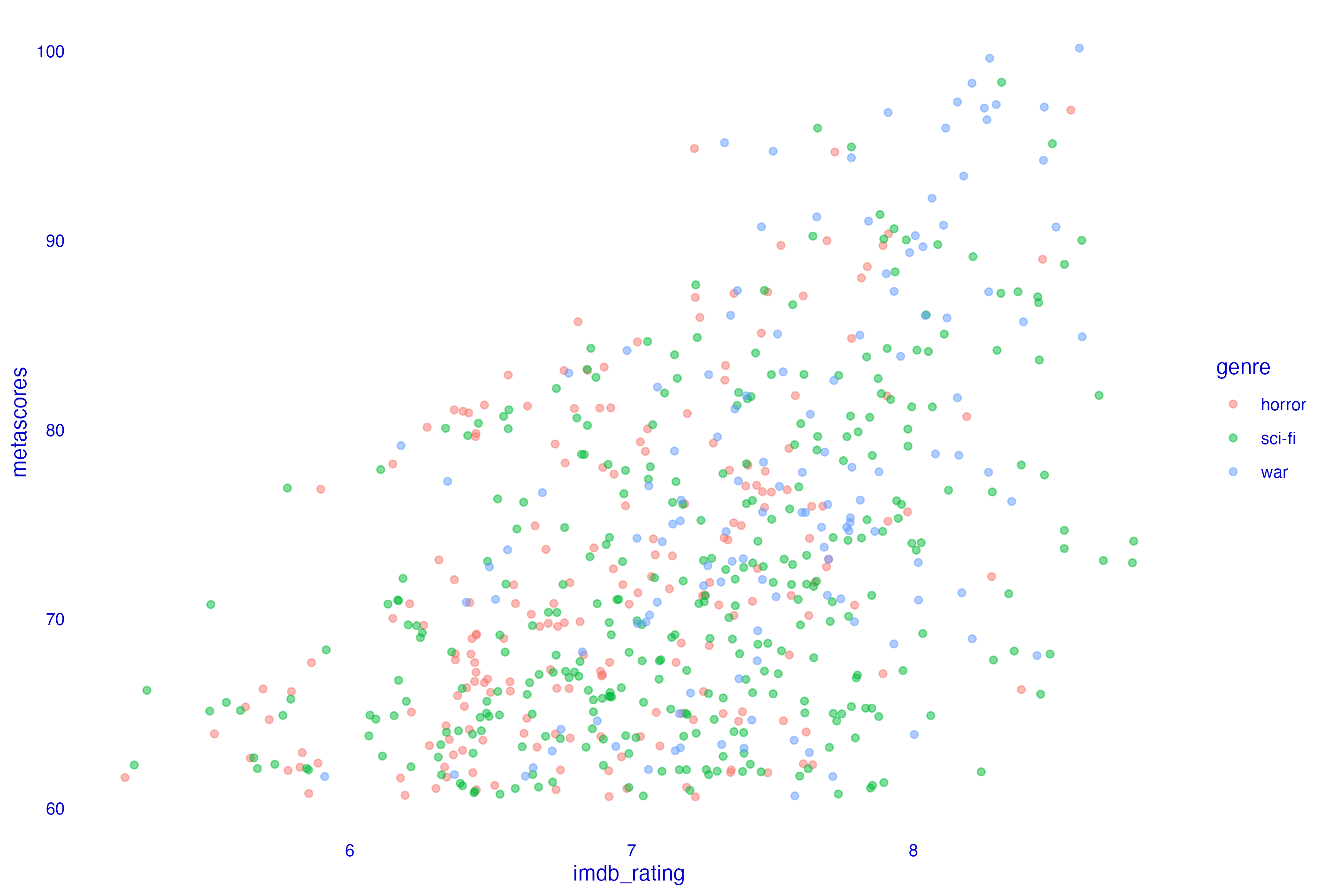
Imagine we wanted to change the axis titles so that they appear blue and emboldened. In this case we need to use a call to element_text(), within which we can manipulate visual parameters like size, colour, alignment and text angle.
# modify plot axis titles
ggplot(imdb_data_clean, aes(x = imdb_rating, y = metascores)) +
  geom_point(aes(colour = genre), position = jitter, alpha = 0.5) +
  theme(axis.title = element_text(face = "bold", colour = "blue"))

Lines in a ggplot2 plot include the tick marks on the axes, the axis lines themselves and all grid lines, both major and minor.

These are also all just arguments within the theme function and are modified by the element_line() function used as an argument to theme().
The remaining non-data elements on our plot are rectangles of various sizes.
Access rectangles using arguments in the theme function and modify them using element_rect().
There is one other important element function that we haven’t discussed yet which is element_blank(). We can use this in a plot to remove any item so that it won’t be drawn at all.
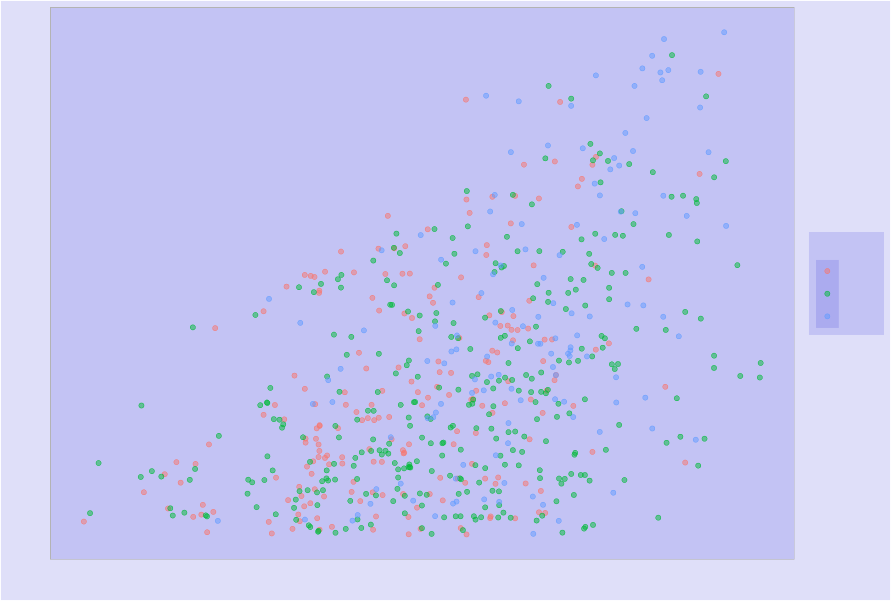
# remove all non-data plot elements
ggplot(imdb_data_clean, aes(x = imdb_rating, y = metascores, colour = genre)) +
  geom_point(position = jitter, alpha = 0.5) +
  theme(
    line = element_blank(),
    rect = element_blank(),
    text = element_blank()
  )
In the example shown below, I have set all lines, text, and rectangles to blank, so we are left with just the data points.
Notice that the legend keys themselves are part of the data, so if you want to modify these elements you will have to modify the aesthetic scales as we spoke about in the previous post.
A Framework for Modifying Themes
The most convenient way to see all the arguments available within the theme layer for modification is to call help for the theme() function by running either help("theme") or ?theme.
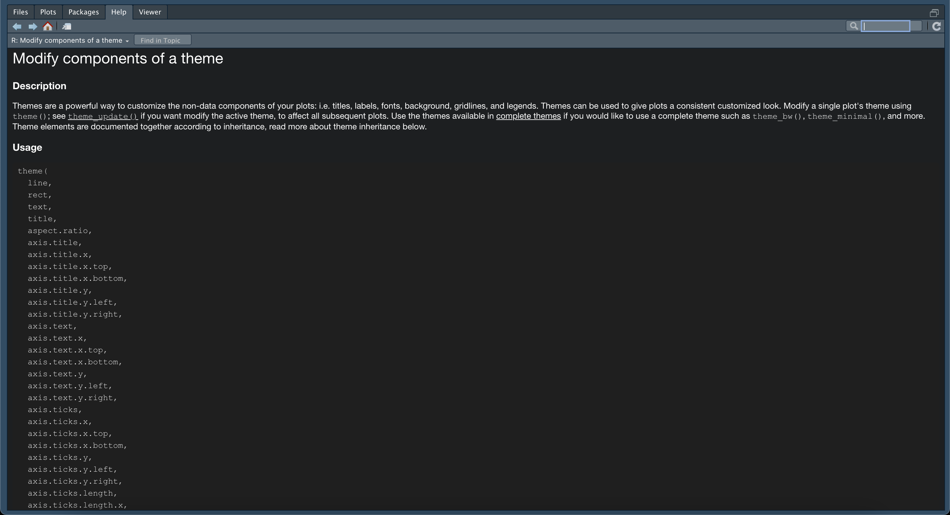
Upon viewing the help page for theme(), as shown in the preview above, you will probably notice a hierarchical inheritance system in place that gives us access to every non-data plot item. For example, all text elements inherit from text, so if we changed that argument, all downstream arguments would be affected. The same goes for line and rect.
Below the top-level arguments, you can access increasingly more specific plot components to make more granular refinements to the plot. For example, using axis.text = element_text() would allow us to modify all axis titles in the same way, but if we only wanted to modify the text for the x axis, we would use axis.text.x = element_text().
Although we have access to every item through theme(), the hierarchical inheritance system means that we don’t need to modify them individually; in practice you will call a small combination of arguments that you want to change.
Let’s go through a more detailed example to consolidate the concepts we have covered so far.
Here’s a moderately customised version of the plot we have been working on:

Here’s the code used to produce the plot. Remember, I am only customising a few of the non-data elements of the plot. If we wanted to customise the actual data points or scales, we would have to follow steps covered in the previous tutorial.
# plot with customised theme elements
ggplot(imdb_data_clean, aes(x = imdb_rating, y = metascores, colour = genre)) +
  geom_point(position = jitter, alpha = 0.5) +
  theme(
    axis.ticks = element_blank(),
    axis.title.x = element_text(margin = margin(10, 0, 0, 0)),
    axis.title.y = element_text(margin = margin(0, 10, 0, 0)),
    legend.title = element_text(face = "bold"),
    legend.title.align = 0.5,
    panel.grid.major = element_line(linetype = "dashed"),
    panel.grid.minor = element_blank(),
    plot.title = element_text(face = "bold")
  ) +
  labs(
    title = "Customised Plot",
    x = "IMDb Rating",
    y = "Metascore",
    colour = "Genre"
  )
Let’s walk through what’s going on here.
The first thing to mention is that I have added a custom labels layer using the labs() function after the theme() call in order to demonstrate a convenient way to do modify the plot, axis and legend titles. These are tasks that most people will want to know how to do and this also allows me to demonstrate how to customise each of the respective plot element in the theme layer.
Moving back to the theme() call itself, I have removed the axis ticks and the minor grid lines for both axes using the element_blank() function with the respective arguments listed in the theme() call. If I had wanted to do this for just one axis or the other I would have used the argument at the next level down in the hierarchy e.g., axis.ticks.x = element_blank() or panel.grid.minor.x = element_blank().
I have customised the text elements that form the various titles I mentioned above with the calls to element_text(). Doing this for the x and y axis titles separately allowed me to modify the margins in a slightly different manner. Borders and margins in ggplot2 require that you use the margin() function to set four positions (top, right, bottom, left) and the units. The default unit is “pt” (points), which scales well with text. Other options include “cm”, “in” (inches) and “lines” (of text).
Finally, I have modified the remaining grid lines with a call to element_line(), setting the linetype to “dashed”. There are various line types available in R, including; “blank”, “solid”, “dashed”, “dotted”, “dotdash”, “longdash” and “twodash”. These line types can be also specified using numbers 0 to 6.
Many plot elements have multiple properties that can be set. For example, line elements have a colour, a thickness (size), and a line type. These parameters can be viewed in the help pages for the respective element function e.g., help("element_line") or ?element_line.
My framework for modifying plot elements in a nutshell is to consult the help for the theme() function, decide which elements you need to modify and the visual element function required to do so, and then consult the help for that function to see how it can be modified. Experiment and have fun making nice, customised plots.
Modifying and Using Themes
Now that we know how to fine-tune every part of our plot using the theme layer, let’s quickly look at a few other useful ways of changing and using theme elements.
1. Defining Theme Layer Objects
If you’re using many plots within a presentation or publication, you’ll want to have consistency in your style. So, once you settle on a specific theme, you’ll want to apply it to all plots of the same type. Creating a theme from scratch is a detailed process that we don’t want to repeat for every plot we make. This is where defining a theme layer object comes into play.
To see how this works, let’s return to the code for the previous plot:
# plot with customised theme elements
ggplot(imdb_data_clean, aes(x = imdb_rating, y = metascores, colour = genre)) +
  geom_point(position = jitter, alpha = 0.5) +

  theme(
    axis.ticks = element_blank(),
    axis.title.x = element_text(margin = margin(10, 0, 0, 0)),
    axis.title.y = element_text(margin = margin(0, 10, 0, 0)),
    legend.title = element_text(face = "bold"),
    legend.title.align = 0.5,
    panel.grid.major = element_line(linetype = "dashed"),
    panel.grid.minor = element_blank(),
    plot.title = element_text(face = "bold")
  ) +

  labs(
    title = "Customised Plot",
    x = "IMDb Rating",
    y = "Metascore",
    colour = "Genre"
  )
As we have seen above, I have changed the axis ticks and titles, the plot and legend titles, and the panel grid lines.
The first method in automating this process would be to save our theme layer as an object. Here I am going to call it theme_imdb
theme_imdb <-
  theme(
    axis.ticks = element_blank(),
    axis.title.x = element_text(margin = margin(10, 0, 0, 0)),
    axis.title.y = element_text(margin = margin(0, 10, 0, 0)),
    legend.title = element_text(face = "bold"),
    legend.title.align = 0.5,
    panel.grid.major = element_line(linetype = "dashed"),
    panel.grid.minor = element_blank(),
    plot.title = element_text(face = "bold")
  )
2. Reusing Theme Objects
Now that we have defined a theme object, we can reuse this style repeatedly. Let’s see what happens when we try to apply our newly defined theme object to another plot.
Here’s the code required to produce a line plot that we made in the previous post.
# data frame of thousands of votes cast for movies by decade and genre
votes_by_decade_genre <- imdb_data_clean %>%
  mutate(decade = 10 * (year %/% 10)) %>%
  group_by(genre, decade) %>%
  summarise(thousands_votes = round(sum(votes)/1e+03))

# base line plot
ggplot(votes_by_decade_genre, aes(x = decade, y = thousands_votes, colour = genre)) +
  geom_line() +
  scale_x_continuous(breaks = seq(from = 1920, to = 2020, by = 10))

Now, all we must do to give it the same theme as our scatter plot is to add the theme_imdb object that we created as a layer instead of having to retype the whole theme layer.
ggplot(votes_by_decade_genre, aes(x = decade, y = thousands_votes, colour = genre)) +
  geom_line() +
  scale_x_continuous(breaks = seq(from = 1920, to = 2020, by = 10)) +
  theme_imdb +
  labs(
    title = "Plot Customised With Reused Theme Object",
    x = "Decade",
    y = "Thousand Votes",
    colour = "Genre"
  )

The only additional change I have made is to update the titles using labs() as we saw how to do earlier.
3. Built-In Themes
A third way of working with themes is accessing the built-in theme templates. Built-in theme functions begin with theme_ and my personal favourite is theme_light(), which makes an excellent template for creating publication-quality plots.
Other built-in themes that you might encounter are:
theme_gray()which is the built-in defaulttheme_classic()a more traditional plot themetheme_bw()andtheme_minimal()which are both similar totheme_light()and useful when using transparencytheme_void()removes everything but the data
There are also add-in packages with pre-defined themes, such as the ggthemes package.
4. Setting and Updating Themes
As you saw at the outset of this tutorial, I set the base plotting theme using the command theme_set(), changing from the automatic default theme_gray() to theme_light(), which looked like this:
# set the base plotting theme
theme_set(theme_light())
If we wanted to create a carbon copy of the default plotting theme (which will be theme_light() if you ran the above code chunk) and then update the same elements that we modified above when creating the theme_imdb object, we could do so using the theme_update() function like so:
# update specific elements of the set theme
theme_update(
  axis.ticks = element_blank(),
  axis.title.x = element_text(margin = margin(10, 0, 0, 0)),
  axis.title.y = element_text(margin = margin(0, 10, 0, 0)),
  legend.title = element_text(face = "bold"),
  legend.title.align = 0.5,
  panel.grid.major = element_line(linetype = "dashed"),
  panel.grid.minor = element_blank(),
  plot.title = element_text(face = "bold")
)
Note that this automatically changes the elements in the set theme, which means your plots will all automatically have these updated elements.
While theme_update() will use the + operator to supersede only the specified elements so that any unspecified values in the theme element will default to the values to which they are set in the theme, the comparable theme_replace() uses the %+replace% operator to completely replace the element. The subtle difference here is that theme_replace() results in unspecified values in the theme element being overwritten with NULL.
There are actually a couple of other advanced ways of modifying themes, such as creating your own theme functions; some of you might have noted earlier on that the theme_imdb object didn’t appear in the code in the same way as the basic theme() layer and that’s because it’s an environmental variable or object and not a function. I will cover these slightly more advanced theming topics in detail in an up-coming intermediate ggplot2 series.
Saving Plots
Now that we have covered aesthetics, geometries, and theming, you’re probably wondering how you can go about saving all the nice plots that you can now make?
Plots can be saved as environmental variables, which can be added to later using the + operator. This is useful if you want to make multiple related plots from a common base plot.
# saving a plot as a variable
base_plot <-
  ggplot(imdb_data_clean, aes(x = imdb_rating, y = metascores, colour = genre)) +
  geom_point(position = jitter, alpha = 0.5)

# re-using a plot saved as a variable
base_plot +
  geom_smooth(method = "lm", se = FALSE) +
  theme_imdb +
  labs(
    title = "Plot Saved as Variable",
    x = "IMDb Rating",
    y = "Metascore",
    colour = "Genre"
  )
Running the above code will save the first plot we made in this tutorial to the object base_plot and then reuses this object to modify the plot further by addition of a second geom layer, application of the theming we saved in our theme_imdb object, and adding a labs() layer, resulting in the plot below.

Saving plots to files in base R used to be a bit of a pain; you had to activate a graphics device while specifying various arguments, run your plotting code, and then switch off the graphics device, which would look something like this:
# not run
png(
  filename = "path/to/file_name.png",
  width = x.xx,
  height = y.yy,
  units = "px",
  ...
)

ggplot(imdb_data_clean, aes(x = imdb_rating, y = metascores, colour = genre)) +
  geom_point(position = jitter, alpha = 0.5)

dev.off()
Each of the different base R graphics devices, of which there are over ten, have a different set of arguments and variable behaviour. Forgetting to run dev.off() was also a frequent cause of issues. Thankfully, ggplot2 provides the convenient ggsave() function, which acts as a unified interface to many of these graphics devices and enables saving of plots with relative ease.
By default, ggsave() uses the last plot that you printed to the plots window, but it can also save those assigned to environmental variables, including objects of classes other than ggplot i.e., those produced by some other plotting packages; pheatmap being a good example that comes to mind as I am writing.
Here’s the equivalent of the above using ggsave() assuming that we had just run the code to preview the plot after writing it.
ggsave(
  filename = "file_name.png",
  device = "png",
  path = "path/to/",
  width = x.xx,
  height = y.yy,
  units = "px",
  ...
)
As you can probably see, there are fewer lines of code, meaning less to go wrong. It also means that there’s much less to learn to save plots, given that you now no longer must know how the arguments for ten or so different graphics device function calls work.
Summary()
Over the course of this introduction to ggplot2 series we have covered the geom layer, mapping variables in your data to aesthetics, modifying aesthetics and scales, and now the theme layer. This means that we’re in a good position to begin a template framework for ggplot2 code:
# required
ggplot(data = DATA, aes(MAPPINGS)) +
  GEOM_FUNCTION(
    stat = STAT,
    position = POSITION
  ) +
# optional
  SCALE_FUNCTION() +
  THEME_FUNCTION()
You now have the ggplot2 core competencies that will allow you to make beautiful and effective exploratory plots but there is a lot more to data visualization and ggplot2: we still need to cover the remaining ggplot2 layers, how to add some embellishments to your plots, intermediate and advanced level ggplot2 trickery, the best of the packages forming the expansive ggplot2 ecosystem and how to use them, and of course, best practices in data visualisation. I will be writing posts or full mini-series on all of these topics, so keep an eye out for these to really round-out your ggplot2 knowledge.
See you next time.
Thanks for reading. I hope you enjoyed the article and that it helps you to get a job done more quickly or inspires you to further your data science journey. Please do let me know if there’s anything you want me to cover in future posts.
Happy Data Analysis!
Disclaimer: All views expressed on this site are exclusively my own and do not represent the opinions of any entity whatsoever with which I have been, am now or will be affiliated.