Introduction
Welcome back to the third part in this step-by-step guide to bulk RNA sequencing data analysis! This tutorial series aims to provide a streamlined bulk RNA-Seq data analysis guided workflow from raw reads to publication-ready figures.
In the first part of this series we processed our raw sequencing (FASTQ) files on a HPC to produce a transcript counts matrix using the gold-standard nf-core/rnaseq pipeline. In part two we read these data into R and carried out a variance stabilising transformation on the data prior to undertaking exploratory and quality control (QC) analyses.
This third part will focus on the differential expression testing elements of the DESeq2 workflow and how to use annotation databases to map between gene-level identifiers. By the end of this tutorial, you should be comfortable performing differential expression testing on pre-processed bulk RNA-Seq gene-level counts data in preparation for downstream pathway and gene set enrichment analyses.
Note: This tutorial is going to continue directly on from part two, so I will be assuming that you have your project directory setup and all of the software and dependencies required installed and loaded. The only object that we need to carry over from last time is the dds object that we created, and we will need to load one additional library for this tutorial later, which is the org.Hs.eg.db package.
Just in case, the requisite DESeqDataSet object for this tutorial can be downloaded as a RDS (R Data Serialization) file from here. Place this into the ./data/processed folder of your project directory tree and read the file by running the code below:
# load dds and res_cln objects
dds <- read_rds(file = here("data", "processed", "dds_backup.rds"))
Now, let’s look at analysing our data.
Differential Expression Testing with DESeq2
The purpose of differential expression testing is to identify genes whose expression levels significantly differ between different experimental conditions, treatments, or groups, providing insights into the molecular mechanisms underlying the biological phenomena being studied.
One important point to raise at the very start here is that DESeq2 requires untransformed and non-normalised counts data as input for the differential expression testing workflow. Although it is a fundamental recommendation to undertake the QC steps that were outlined in the last tutorial, and these require that the data are transformed (e.g., using a variance stabilising transformation), this transformation is not required prior to differential expression testing using DESeq2. For further information, see the DESeq2 vignette.
Using the raw counts matrix (taken directly from the DESeqDataSet) as input, the DESeq2 workflow undertakes three main computations as part of the differential expression testing process before we can draw contrasts from our biological conditions of interest: estimation of size factors, estimation of dispersion parameters, and then fitting of the statistical model for determination of differential expression.
Before we start working on our data, let’s create a test data set to demonstrate the inner workings of this set of computations before we start using them on our data.
# create a small counts matrix for two samples to demonstrate DESeq2 workflow
demo_data <-
  matrix(
    data = c(1489, 22, 793, 76, 521, 906, 13, 410, 42, 1196),
    nrow = 5,
    dimnames = list(
      c("GAPDH","ACTB","B2M","HPRT1","RPL13A"),
      c("sample_1","sample_2")
    )
  )
Now, let’s take a detailed look at the DESeq2 differential expression workflow.
Estimation of Size Factors
The first computation undertaken on the raw count matrix within the DESeqDataSet object is estimation of the size factors for each sample in an RNA-Seq dataset.
Size factors are scaling factors that normalise the raw read counts to account for differences in sequencing depth and other technical biases across samples. This normalisation step is crucial to ensure that the comparisons of gene expression levels between samples are accurate and not confounded by technical variability.
Size factors are calculated based on the median ratio of gene counts relative to a gene-wise pseudo-reference sample (the gene-wise geometric mean across all samples), which helps in achieving a comparable scale across all samples in the dataset.
The estimateSizeFactors() function can be used to undertake this computation. The following code chunk uses our demonstration data set to shows the sequential calculations that estimateSizeFactors() undertakes in the background.
# calculate row-wise geometric mean pseudo-reference
psuedo_ref <- sqrt(rowProds(demo_data))

# calculate ratio of each sample to the reference
ratios <- divide_by(demo_data, psuedo_ref)

# calculate the normalisation factor for each sample
norm_factors <- colMedians(ratios)

# normalise each sample in the data set
norm_data <- sweep(demo_data, 2, norm_factors, divide_by)

# print the matrices pre- and post-normalisation
print(demo_data)
print(norm_data)
> print(demo_data)
       sample_1 sample_2
GAPDH      1489      906
ACTB         22       13
B2M         793      410
HPRT1        76       42
RPL13A      521     1196

> print(norm_data)
         sample_1   sample_2
GAPDH  1144.60340 1178.60387
ACTB     16.91153   16.91153
B2M     609.58395  533.36378
HPRT1    58.42166   54.63727
RPL13A  400.49589 1555.86118
We can see the effect that this normalisation has on the demonstration data set; the gene-wise counts between samples have been adjusted for the differences in technical variability, ensuring that any subsequent analyses are based on biologically relevant differences rather than technical artifacts. We can visualise these changes in the overall count distribution of each sample pre- and post-normalisation using a box and whisker plot; I have not provided the code for this as it is purely for demonstrative purposes.
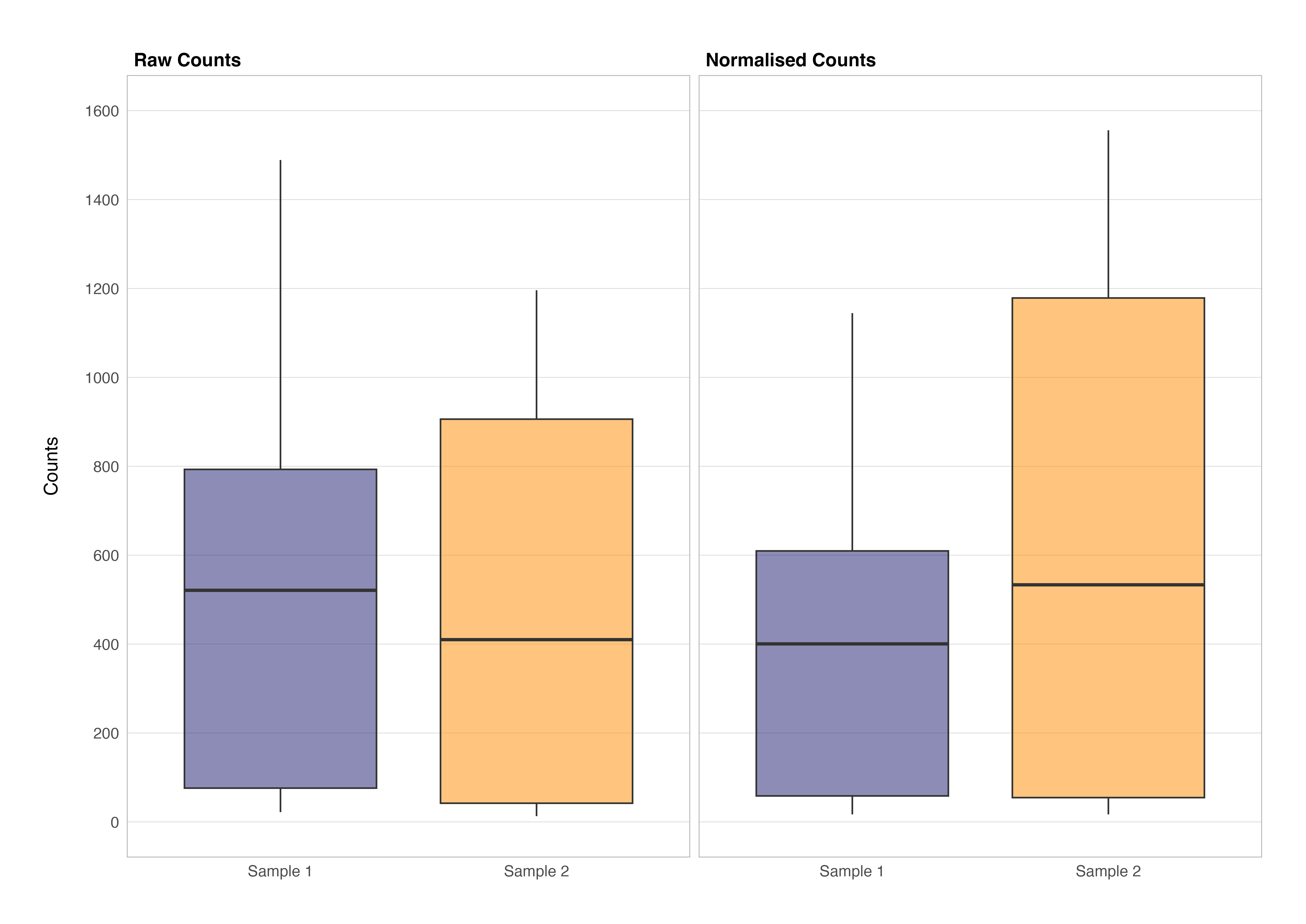
It is clear from looking at the data and plot above that if normalisation was not undertaken, incorrect conclusions around the magnitude and distribution of gene-wise counts for sample 2 could be drawn. For example, one might falsely conclude that GAPDH is more lowly expressed in sample 2 than sample 1 when in fact we can see this is not the case.
DESeq2 has a single estimateSizeFactors() function that we can use to generate size factors for us and perform median of ratios normalisation. Assigning the output of this function back to our DESeqDataSet object dds will allow us to do three important things.
First, it allows us to view the normalisation factor applied to each sample.
# undertake median of ratios normalisation
dds <- estimateSizeFactors(dds)

# view the normalisation factor applied to the data
colData(dds)
sizeFactors(dds)
> colData(dds)
DataFrame with 9 rows and 6 columns
           assay_name              phenotype   sample_id    group      rep sizeFactor
          <character>            <character> <character> <factor> <factor>  <numeric>
ctr_bc_2   1_CTR_BC_2                control    ctr_bc_2      CTR        1   1.062897
tgf_bc_4   2_TGF_BC_4 TGF-beta-1 induced m..    tgf_bc_4      TGF        1   1.179409
ir_bc_5     3_IR_BC_5 gamma irradiation in..     ir_bc_5      IR         1   0.882836
ctr_bc_6   4_CTR_BC_6                control    ctr_bc_6      CTR        2   1.097633
tgf_bc_7   5_TGF_BC_7 TGF-beta-1 induced m..    tgf_bc_7      TGF        2   1.050744
ir_bc_12   6_IR_BC_12 gamma irradiation in..    ir_bc_12      IR         2   0.846937
ctr_bc_13 7_CTR_BC_13                control   ctr_bc_13      CTR        3   0.952185
tgf_bc_14 8_TGF_BC_14 TGF-beta-1 induced m..   tgf_bc_14      TGF        3   1.071315
ir_bc_15   9_IR_BC_15 gamma irradiation in..    ir_bc_15      IR         3   0.968518

> sizeFactors(dds)
 ctr_bc_2  tgf_bc_4   ir_bc_5  ctr_bc_6  tgf_bc_7  ir_bc_12 ctr_bc_13 tgf_bc_14  ir_bc_15
1.0628974 1.1794091 0.8828362 1.0976331 1.0507445 0.8469367 0.9521847 1.0713154 0.9685181
Second, it enables us to extract and write-out the normalised counts matrix for later use e.g., visualisations that require normalised counts, such as an expression plot.
# extract normalised counts
norm_counts <- counts(dds, normalized = TRUE)
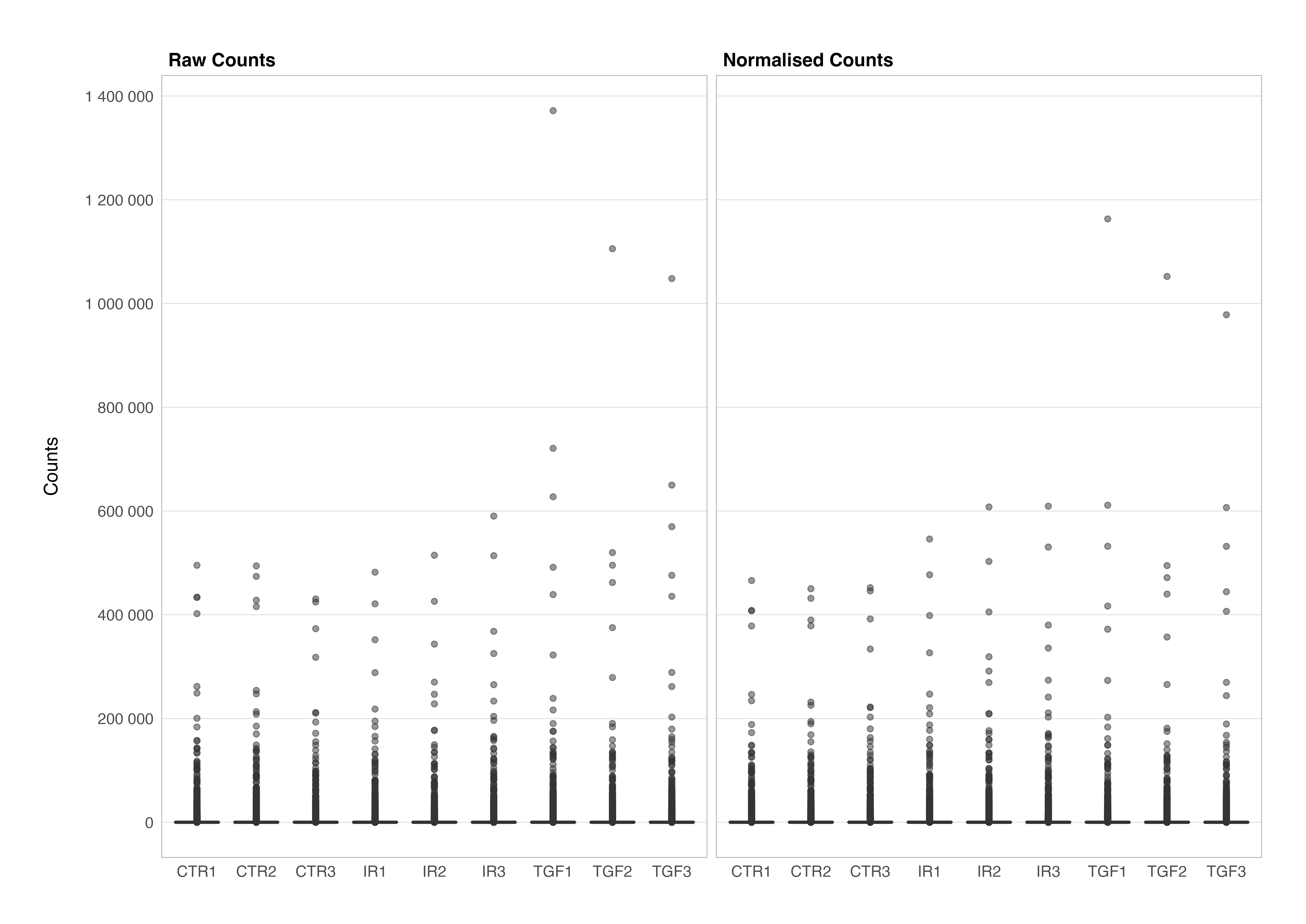
Finally, it allows us to visualise the raw and normalised counts in our experimental data set in the same way that we have just done for our demo data; not strictly necessary if you trust the process but nothing beats seeing that something has worked with your own eyes. Again, code not included as this graph is shown for demonstration purposes.
One final thing to note is that, unlike the trimmed mean of M values (TMM) normalisation method used in the edgeR package, the median of ratios normalisation method in DESeq2 does not account for differences in gene lengths. This is because, differential expression analysis compares the counts between sample groups for the same gene, therefore the gene length does not need to be accounted for, while sequencing depth and RNA composition do need to be considered.
Estimation of Dispersion
After normalising using the median of ratios method, the next step in the DESeq2 workflow is estimating the dispersion parameters for each gene in the RNA-Seq dataset.
Dispersion measures the variability of gene expression levels across biological replicates beyond what is expected from Poisson variation alone. DESeq2 uses a specific measure of dispersion that is related to both the mean and variance of gene counts.
Accurate estimation of dispersion is crucial for differential expression analysis because it accounts for biological variability and technical noise in the data. To accurately model sequencing counts, DESeq2 needs reliable estimates of within-group variation (variation between replicates of the same sample group) for each gene. With few replicates per group, these estimates are often unreliable due to large differences in dispersion for genes with similar means.
To address this, DESeq2 shares information across genes to generate more accurate estimates of variation based on the mean expression level of the gene using a method called shrinkage. DESeq2 assumes that genes with similar expression levels have similar dispersion values.
The dispersion estimation process in DESeq2 involves several steps:
-
Initial Estimation: Dispersion for each gene is initially estimated using maximum likelihood estimation (MLE). Given the count values of the replicates, the most likely estimate of dispersion is calculated.
-
Fitting a Dispersion Trend: A trend is fitted to the dispersion estimates as a function of the mean expression level. This trend captures the overall relationship between gene expression levels and their variability, acknowledging that different genes have different scales of biological variability but generally follow a predictable pattern.
-
Shrinkage to the Trend: The initial dispersion estimates are then shrunk towards the fitted trend. This shrinkage step borrows strength across genes, resulting in more stable and reliable dispersion estimates, especially for genes with few replicates or low counts.
The combination of these steps, which is undertaken by the estimateDispersions() function in DESeq2, ensures that the dispersion estimates used in subsequent differential expression testing are robust and account for both biological and technical variability in the RNA-Seq data.
# dispersion estimation
dds <- estimateDispersions(dds)
gene-wise dispersion estimates
mean-dispersion relationship
final dispersion estimates
The model fit during dispersion estimation is displayed as a red line in the figure shown below, which is a plot of the estimate for the expected dispersion value for genes at a given expression level; each black dot is a gene with an associated mean expression level and maximum likelihood estimation of the dispersion, each blue dot is the final estimate following shrinkage to the fitted trend. It’s worth noting here that you don’t have to show-off and build this plot from scratch using ggplot2 as I have done; a perfectly serviceable rudimentary version can be produced by running plotDispEsts(dds).
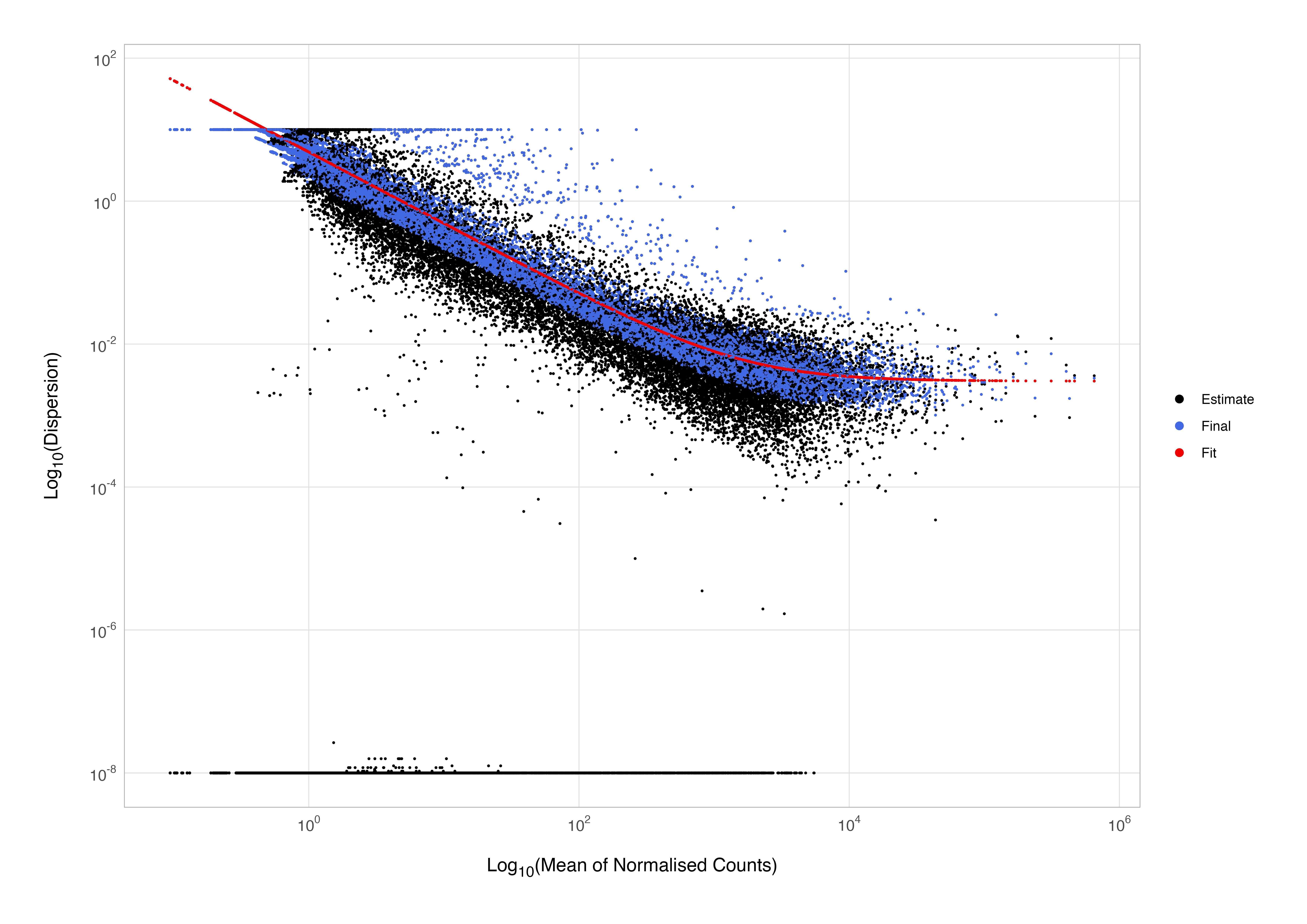
This plot is great for ensuring your data are a good fit for the DESeq2 model; we might expect our data to generally scatter around the curve, with the dispersion decreasing with increasing mean expression levels. If you see a cloud or different shapes here, then you might want to explore your data more to see if you have contamination (e.g., high levels of mitochondrial genes due to dead/dying cells) or outlier samples.
Model Fitting and Hypothesis Testing
The final step in the DESeq2 workflow is fitting a model for each gene and performing differential expression testing.
DESeq2 fits a generalised linear model (GLM) to the count data for each gene, where the counts are assumed to follow a negative binomial distribution. This distribution accounts for both the mean and the dispersion of the counts, accommodating the overdispersion typically observed in RNA-Seq data (i.e., the variance exceeding the mean).
The null hypothesis for differential expression testing states that there is no differential expression across the conditions of interest, i.e., the log2 fold-change between conditions is zero. DESeq2 uses the Wald test (by default) to test this hypothesis. The Wald test evaluates the significance of coefficients in the fitted model. Specifically, it tests whether the log2 fold-change estimate for each gene is significantly different from zero.
The Wald test for data assumed to follow a negative binomial distribution is undertaken in DESeq2 using the nbinomWaldTest() function.
# perform wald test for data following negative binomial distribution
dds <- nbinomWaldTest(dds)
The Wald test statistic is calculated for each gene, and a corresponding p-value is computed. The p-value indicates the probability of observing a test statistic as extreme as, or more extreme than, the one calculated, under the null hypothesis.
- Null Hypothesis (H0): The gene is not differentially expressed (log2 fold-change = 0).
- Alternative Hypothesis (H1): The gene is differentially expressed (log2 fold-change ≠ 0).
If the p-value is small (typically less than a chosen significance level, such as 0.05), the null hypothesis is rejected, providing evidence that the gene is differentially expressed between conditions.
Putting It All Together
So far we have seen that differential expression testing in DESeq2 requires that we run three functions on the DESeqDataSet object dds that we constructed in the previous tutorial, in the order shown below. We can, of course, use pipes with this series of commands as an alternative to assigning the intermediate outputs back to dds.
# create the DESeq2 data set object (reminder)
dds <-
  DESeqDataSetFromMatrix(
    countData = count_matrix,
    colData = meta_data_cln,
    design = ~group
  )

# step-wise differential expression testing (example only: do not run)
dds <- estimateSizeFactors(dds)
dds <- estimateDispersions(dds)
de <- nbinomWaldTest(dds)

# differential expression testing as a pipeline (example only: do not run)
de <-
  dds %>%
  estimateSizeFactors() %>%
  estimateDispersions() %>%
  nbinomWaldTest()
Luckily, rather than having to remember these three functions and their sequential order, there is a convenient function DESeq() that will run all of these for us and print out messages to remind us of the steps being undertaken.
# one function to control them all and in the darkness bind them
de <- DESeq(dds)
estimating size factors
estimating dispersions
gene-wise dispersion estimates
mean-dispersion relationship
final dispersion estimates
fitting model and testing
There are many arguments which can be used to configure the behaviour of this function (including using an alternative hypothesis test - the likelihood ratio test), a deep dive on which are outside the scope of this tutorial. You can read more about this in the DESeq2 vignette.
If you print the de object that we have just created, you will notice that the results of the analysis are not immediately accessible; we still have a DESeqDataSet object.
class: DESeqDataSet
dim: 63241 9
metadata(1): version
assays(4): counts mu H cooks
rownames(63241): ENSG00000000003 ENSG00000000005 ... ENSG00000293559 ENSG00000293560
rowData names(26): baseMean baseVar ... deviance maxCooks
colnames(9): ctr_bc_2 tgf_bc_4 ... tgf_bc_14 ir_bc_15
colData names(6): assay_name phenotype ... rep sizeFactor
To access the differential expression testing result for each gene in our data set, we have to call the results() function. This function extracts a result table from the DESeq analysis giving base means across samples, log2 fold changes, standard errors, test statistics, p-values and adjusted p-values. The final point is an important one; given that thousands of genes are tested simultaneously, the results function in DESeq2 applies multiple testing correction to control the false discovery rate (FDR) using the Benjamini-Hochberg procedure by default.
# obtain differential expression testing results
results(de)
log2 fold change (MLE): group TGF vs CTR
Wald test p-value: group TGF vs CTR
DataFrame with 63241 rows and 6 columns
                   baseMean log2FoldChange     lfcSE       stat     pvalue      padj
                  <numeric>      <numeric> <numeric>  <numeric>  <numeric> <numeric>
ENSG00000000003 1345.455780      -0.231992 0.0822977 -2.8189413 0.00481823 0.0209020
ENSG00000000005    0.114723      -0.085745 4.0804559 -0.0210136 0.98323483        NA
ENSG00000000419 1820.021529      -0.140142 0.0954316 -1.4685019 0.14196794 0.2903151
ENSG00000000457  547.278623      -0.294895 0.1146352 -2.5724659 0.01009769 0.0377053
ENSG00000000460  194.507613       0.161109 0.1671488  0.9638653 0.33511344 0.5265196
...                     ...            ...       ...        ...        ...       ...
ENSG00000293556    2.691654       0.304377   1.47936  0.2057485   0.836987        NA
ENSG00000293557    1.256348       2.795721   2.35008  1.1896266   0.234193        NA
ENSG00000293558    0.417864       1.683934   4.04595  0.4162021   0.677262        NA
ENSG00000293559    0.125857      -0.085745   4.08046 -0.0210136   0.983235        NA
ENSG00000293560    0.629229       0.784454   3.44541  0.2276805   0.819895        NA
Note that all genes are reported in the output of the call to results(), not just the significant ones. There are some other issues with this output that we can address too. More on this shortly.
Experimental Design and Contrasts
You may have noted when looking at the output above, that the information in the header gives us some information about the two groups in our data that have been compared during the differential expression test to which the results pertain; this is called a contrast. More formally, a contrast is a linear combination of estimated log2 fold changes, which can be used to test if differences between groups are equal to zero.
The contrasts that are available for testing will depend on the experimental design which was specified by the design argument when we created the dds DESeqDataSet object. The design tells DESeq2 which variable(s) in the sample metadata can be used to specify the groups of interest to compare and any interaction terms for differential expression analysis. For a detailed overview of these topics, consult the DESeq2 vignette.
Typically, we decide the design for the analysis when we create DESeqDataSet objects, but it can be accessed to check the design that has been specified, and modified if required, prior to the differential expression analysis using the design() function.
# check specified experimental design
design(dds)

# modify the experimental design (example only: do not run)
design(dds) <- ~foo
In our case, we have indicated that we wish to draw a contrast based on the group variable in the experimental metadata, and as we have encoded this as a factor with three levels CTR, IR and TGF, there are several potential contrasts that we could draw e.g., CTR vs IR, CTR vs TGF and IR vs TGF. The resultsNames() function can be used to indicate the contrasts (model coefficients) that can be accessed under the experimental design that has been specified.
# view available model coefficents
resultsNames(de)
In the analysis that we have undertaken, DESeq2 has automatically decided which member of our sample groups to use as our baseline condition (CTR in this case) and the log2 fold-changes in the results that are positive indicate that the respective gene is more highly expressed in the TGF group than CTR.
In order to specify the contrast variable that we wish to use, or change the directionality of that contrast, we can use the contrast argument to the results() function, as shown here.
# change the direction of the default contrast
results(de, contrast = c("group", "CTR", "TGF"))

# change the experimental conditions in the contrast
results(de, contrast = c("group", "IR", "CTR"))
All the above examples perform a differential expression analysis using a single named column in the metadata slot of the dds object. However, DESeq2 can performing much more complex analyses based on multiple experimental factors, so-called multi-factor designs. One potential motivator for the use of such a design might be the discovery of a batch effect in the data, such as that shown in the simulated example below which we have seen in the previous tutorial.
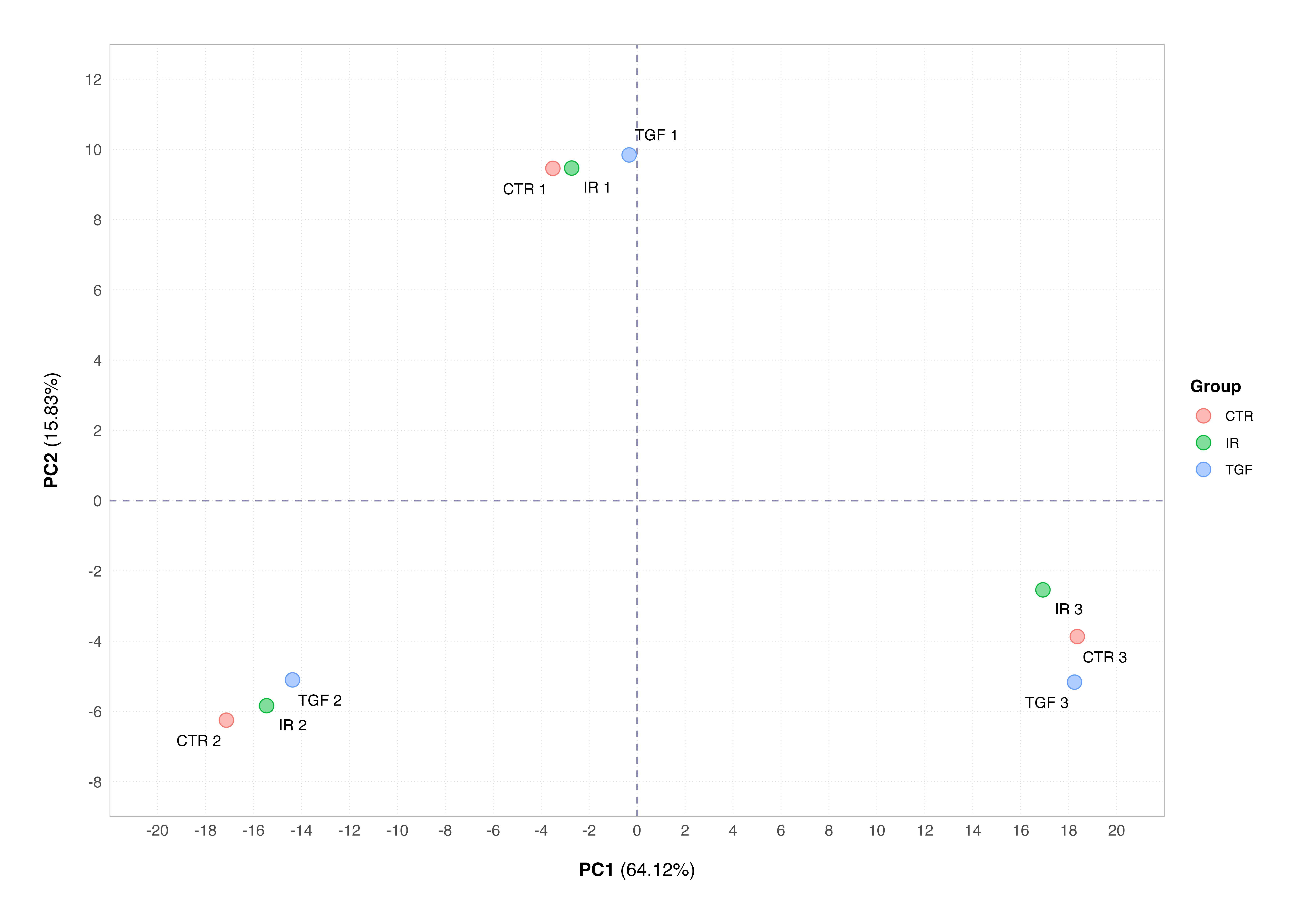
Rather than removing this batch effect by adjusting the read counts prior to constructing the dds object (as you might do using the SVA package), we can simply incorporate the batch into the experimental design.
# modify the experimental design (example only: do not run)
design(dds) <- ~rep + group
While adjusting batch effects using external packages like SVA allows for clear visualisation of batch correction via pre- and post-correction PCA plots and simplifies downstream models, not everyone is going to need to isolate this technical noise explicitly. In many cases, the simpler, equally robust and more widely used approach of integrating batch effects directly into the design matrix of the differential expression analysis will suffice.
An important point to note is that the order here matters; the design shown above specifies that the main effect we are interested in is group while controlling for rep i.e., the technical replicate. If we had written this as ~group + rep it would mean that we would control for group and the main effect on which differential expression testing would be undertake would be the rep variable.
One final point is that both solutions to controlling for batch effect assume that representatives of the groups of interest appear in each batch, and that batches aren’t confounded by another variable of interest e.g., cell line.
A more detailed discussion of DESeq2 designs and these issues is beyond the scope of this tutorial. For a more detailed discussion of this topics, consult the DESeq2 vignette or checkout this video tutorial.
Processing Results Using Tidyverse
As I mentioned just before we looked at experimental designs, the output of the call to the results() function reports the results for all genes in our counts matrix, not just the significant ones. In addition, the gene identifiers (Ensembl gene IDs) by which rows are currently ordered are not very informative, and the format of the output (and more specifically the object class) is not compatible with standard data manipulation tools (i.e., tidyverse packages and functions).
Let’s start with the low-hanging fruit. The results function has an argument which can be used to coerce the default DESeqResults object returned to a tidy data frame. To make it even more tidyverse compatible, we can then convert this to a tibble.
# obtain tidyverse-compatible DE testing results
res <-
  results(de, contrast = c("group", "IR", "CTR"), tidy = TRUE) %>%
  tibble()

# preview results
print(res)
# A tibble: 63,241 × 7
   row             baseMean log2FoldChange  lfcSE   stat        pvalue          padj
   <chr>              <dbl>          <dbl>  <dbl>  <dbl>         <dbl>         <dbl>
 1 ENSG00000000003 1345.           -0.138  0.0828 -1.67  0.0946         0.235
 2 ENSG00000000005    0.115         1.17   4.08    0.286 0.775         NA
 3 ENSG00000000419 1820.            0.256  0.0953  2.69  0.00724        0.0300
 4 ENSG00000000457  547.           -0.0870 0.115  -0.757 0.449          0.665
 5 ENSG00000000460  195.           -1.07   0.181  -5.93  0.00000000303  0.0000000493
 6 ENSG00000000938    6.83         -0.723  0.968  -0.747 0.455          0.670
 7 ENSG00000000971 4744.           -0.142  0.0592 -2.40  0.0163         0.0588
 8 ENSG00000001036 3438.            0.184  0.0570  3.24  0.00120        0.00654
 9 ENSG00000001084  869.            0.0837 0.0954  0.878 0.380          0.603
10 ENSG00000001167 1292.           -0.223  0.0935 -2.39  0.0170         0.0606
# ℹ 63,231 more rows
# ℹ Use `print(n = ...)` to see more rows
You will notice that the output no longer shows a header detailing the contrast used, and that gene IDs are now a variable row as opposed to being used as row names. We can improve this output further by adding additional gene-level annotation and wrangling the data a little to make the formatting more user-friendly i.e., ready for sharing with group members or collaborators.
There are many packages available withing the Bioconductor ecosystem in R for annotating biological data; these are listed in the AnnotationData section. As such, there are several possible ways to add annotation to our data. One popular approach is to use the biomaRt package, an API for access to BioMart databases. These tools, while comprehensive, may seem a little daunting to the uninitiated.
We will take a simpler approach here and add annotation using the AnnotationDbi and org.Hs.eg.db packages; the latter being one of several off-line SQLite database packages in Bioconductor that are re-built every six months offering organism-level access to genome-wide annotation.
Once we have loaded the package, we first need to identify what information is available to us and which variables we want to add to our data.
# load package
library(org.Hs.eg.db)

# view db variables
columns(org.Hs.eg.db)
[1]  "ACCNUM"       "ALIAS"        "ENSEMBL"      "ENSEMBLPROT"  "ENSEMBLTRANS" "ENTREZID"     "ENZYME"
[8]  "EVIDENCE"     "EVIDENCEALL"  "GENENAME"     "GENETYPE"     "GO"           "GOALL"        "IPI"
[15] "MAP"          "OMIM"         "ONTOLOGY"     "ONTOLOGYALL"  "PATH"         "PFAM"         "PMID"
[22] "PROSITE"      "REFSEQ"       "SYMBOL"       "UCSCKG"       "UNIPROT"
To build our annotation data frame, we first need to filter the database using a set of keys to extract the specific information that we want in relation to each gene within our results data frame. For routine bulk RNA-Seq analysis, I usually only add SYMBOL (HUGO gene symbols) and GENENAME gene names to make the gene IDs human readable, along with ENTREZID (Entrez gene IDs) which are required by the various tools used in gene set enrichment analyses. We know that we have Ensembl IDs in our data set already, so we will use this as the key type to access the information we need, and we will extract the information related to each key or individual Ensembl ID. The final thing that we will specify is the columns or variables within the database from which we want to retrieve this gene-level information.
# create annotation
annot_df <-
  AnnotationDbi::select(
    org.Hs.eg.db,
    keys = rownames(dds), # could use res$row here
    keytype = "ENSEMBL",
    columns = c("ENTREZID", "SYMBOL", "GENENAME")
  )
One thing to note here is that the select() function must be called from the AnnotationDbi namespace, to avoid errors resulting from an attempt to call the dplyr function of the same name. Once you execute the above chunk, you will receive the following warning:
'select()' returned 1:many mapping between keys and columns
This occurs because there are often several different identifiers from other annotations used for each Ensembl ID. We will deal with this issue shortly. Let’s preview the annotation data frame that we have created. The results will be returned in the order which the keys were in when the query was run, which will be the alphanumeric order of our Ensembl IDs by default.
# preview annotation
head(annot_df, n = 10)
           ENSEMBL ENTREZID SYMBOL                                                    GENENAME
1  ENSG00000000003     7105 TSPAN6                                               tetraspanin 6
2  ENSG00000000005    64102   TNMD                                                 tenomodulin
3  ENSG00000000419     8813   DPM1 dolichyl-phosphate mannosyltransferase subunit 1, catalytic
4  ENSG00000000457    57147  SCYL3                                    SCY1 like pseudokinase 3
5  ENSG00000000460    55732  FIRRM   FIGNL1 interacting regulator of recombination and mitosis
6  ENSG00000000938     2268    FGR              FGR proto-oncogene, Src family tyrosine kinase
7  ENSG00000000971     3075    CFH                                         complement factor H
8  ENSG00000001036     2519  FUCA2                                        alpha-L-fucosidase 2
9  ENSG00000001084     2729   GCLC                 glutamate-cysteine ligase catalytic subunit
10 ENSG00000001167     4800   NFYA                nuclear transcription factor Y subunit alpha
We can easily determine how many duplicate entries there within our data frame (3992 in this case) and then remove these; there are several ways to do these tasks, but I prefer to use simple tidyverse syntax where possible over base R syntax.
# determine number of duplicate entries
sum(duplicated(annot_df$ENSEMBL))

# remove duplicates
annot_dup_rm <- distinct(annot_df, ENSEMBL, .keep_all = TRUE)
Now all that’s left to do before we are ready to save the results is to join this information on to our results data frame and do a little data wrangling to make the final output as user-friendly as possible. After this, we can easily determine the number of significant results at a specific significance cut-off value and filter the cleaned results data frame to return the genes with significant FDR-adjusted p-values.
Note: Some will also want to incorporate a log2fold-change cut-off here; it is more desirable (from a statistical standpoint in terms of correctly controlling the type-I error rate) to incorporate this threshold into the hypothesis test and then filter for significant results than it is to apply this log2fold-change threshold as a post-hoc filtration step. This is exactly what I am going to do below prior to adding our annotation. For more information, checkout the specific section in the DESeq2 vignette.
# test for de using lfc threshold
res <-
  results(
    de,
    contrast = c("group", "IR", "CTR"),
    tidy = TRUE,
    lfcThreshold = 1,
    altHypothesis = "greaterAbs",
    pAdjustMethod = "BH"
  ) %>%
  tibble()

# wrangle results and add annotation
res_cln <-
  res %>%
  left_join(annot_dup_rm, by = c("row" = "ENSEMBL")) %>%
  janitor::clean_names() %>%
  relocate(entrezid:genename, .after = row) %>%
  rename(all_of(c(ensembl = "row", entrez = "entrezid", lfc = "log2fold_change"))) %>%
  filter(!is.na(padj)) %>%
  arrange(padj)

# number of significant results
count(res_cln, signif = padj < 0.05, name = "count")

# filter results
sig_res <- filter(res_cln, padj < 0.05)

# preview the cleaned significant results
print(sig_res)
# A tibble: 238 × 10
   ensembl         entrez symbol genename                                 base_mean   lfc lfc_se  stat   pvalue     padj
   <chr>           <chr>  <chr>  <chr>                                        <dbl> <dbl>  <dbl> <dbl>    <dbl>    <dbl>
 1 ENSG00000183801 283298 OLFML1 olfactomedin like 1                           577. -2.76 0.139  -19.9 2.68e-37 5.42e-33
 2 ENSG00000225783 440823 MIAT   myocardial infarction associated transc…      501. -2.58 0.140  -18.5 5.55e-30 5.62e-26
 3 ENSG00000116774 56944  OLFML3 olfactomedin like 3                          4128. -1.78 0.0704 -25.3 4.72e-29 3.19e-25
 4 ENSG00000148773 4288   MKI67  marker of proliferation Ki-67                1493. -1.98 0.0906 -21.9 8.15e-28 4.13e-24
 5 ENSG00000107562 6387   CXCL12 C-X-C motif chemokine ligand 12              5245. -2.99 0.190  -15.8 4.10e-26 1.66e-22
 6 ENSG00000113368 4001   LMNB1  lamin B1                                      692. -2.63 0.159  -16.5 7.85e-25 2.65e-21
 7 ENSG00000131747 7153   TOP2A  DNA topoisomerase II alpha                   4403. -2.15 0.115  -18.7 6.66e-24 1.93e-20
 8 ENSG00000046653 2824   GPM6B  glycoprotein M6B                              252. -2.94 0.195  -15.1 1.22e-23 3.09e-20
 9 ENSG00000186469 54331  GNG2   G protein subunit gamma 2                     843. -2.16 0.124  -17.4 4.66e-21 1.05e-17
10 ENSG00000112984 10112  KIF20A kinesin family member 20A                    1012. -2.05 0.117  -17.5 1.44e-19 2.91e-16
# ℹ 228 more rows
# ℹ Use `print(n = ...)` to see more rows
We can see from the output shown above that at an FDR-adjusted p-value of < 0.05 there are 238 genes differentially expressed between irradiated and control groups above a log2 fold-change threshold of 1 (abs. log2 fold-change of 2 or more).
The more experienced amongst those of you reading this may have noticed that at no point have I undertaken nor discussed pre-filtration of the counts data. This is because it is not actually required in DESeq2, though you will often see it as part of many workflows; it has its advantages and disadvantages, which I won’t discuss here. That is not to say that genes with low counts were not accounted for in our workflow. The results() function applies an independent filter to the mean of normalised counts, and the adjusted p-values for the genes which did not pass the filter threshold were automatically set to NA and filtered out (using the filter(!is.na(padj)) step) during our results cleaning and wrangling. That is to say, I intentionally omitted pre-filtration in favour of the independent filtering procedures available within DESeq2. For more detail on these topics, please consult the relevant sections in the DESeq2 vignette.
It would be sensible at this point to perform a final “sanity” check and plot the sample-level counts for genes with high significance. Similarly, if your study involves knocking-out a particular gene, or you have some positive controls that are known in advance, it would be a good idea to visualise their expression levels across conditions within a contrast. The DESeq2 package contains a convenient plotCounts() function for this purpose; the output is not particularly attractive but is a good quick-and-dirty plot for diagnostic purposes.
# sample-level counts for a highly significant result
plotCounts(dds, gene = "ENSG00000183801", intgroup = "group")
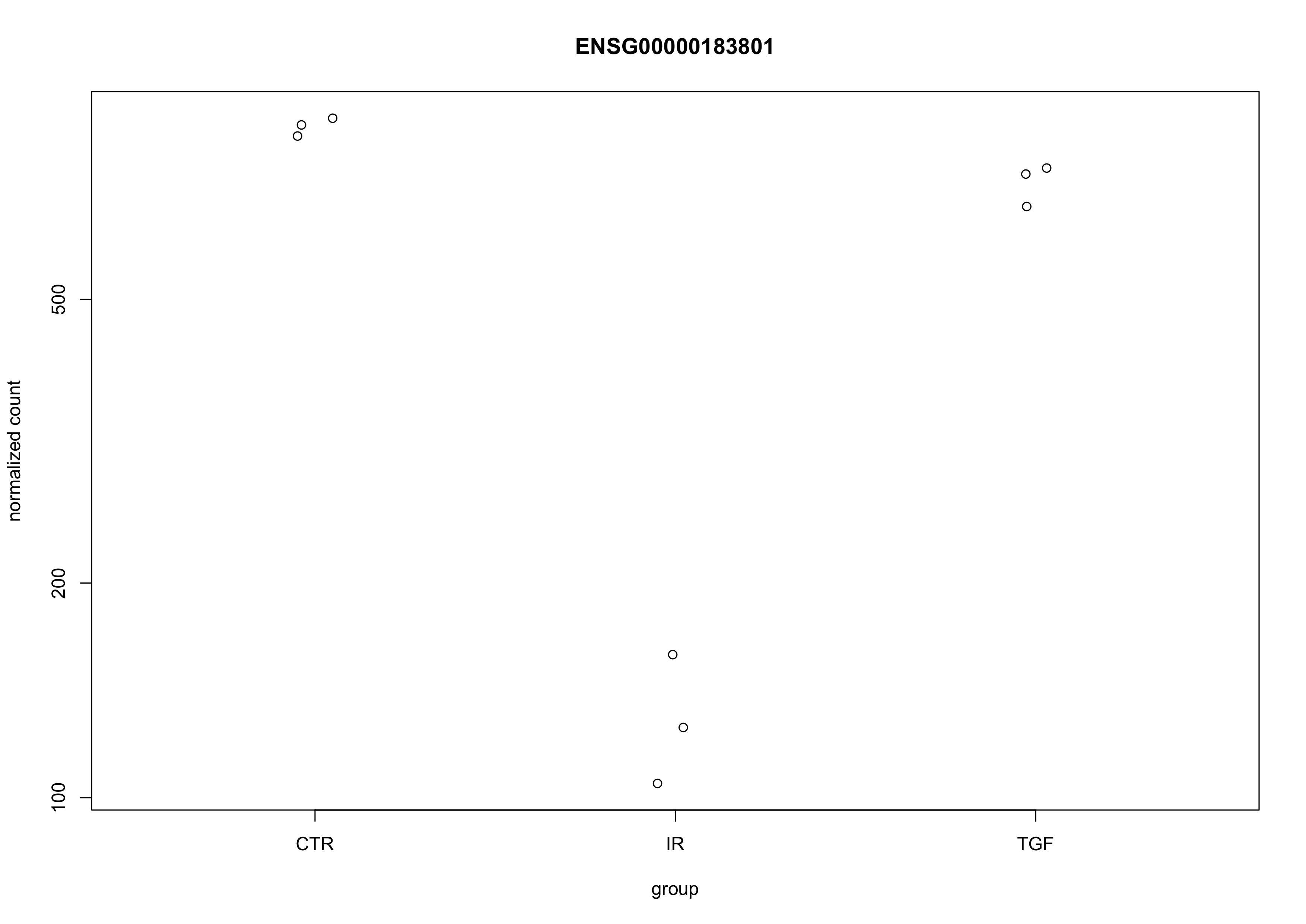
The Ensembl IDs that I have picked here is that for OLFML1, the most significant result in the head of the results data frame displayed above. As we can clearly see, the normalised counts values (stored in the assay slot of the dds DESeqDataSet object) are much lower in the radiation-treated group than the control group, corresponding with the log2 fold-change of -2.76 shown in the data (which we can approximate from the graph as log2(120) - log2(800) = -2.73). This all looks good to me. At this point, we could write-out our cleaned and filtered results, safe in the knowledge that everything makes sense.
# write out results
write_csv(res_cln, file = here("results", "tables", "ir_vs_ctr_all.csv"))
Now that we have conducted differential expression testing and saved our results, it’s time for a victory brew ☕
Summary
That’s it for the fundamentals of differential expression testing in DESeq2! You are now equipped with the essential skills required to run your own analyses and have been signposted to all the resources required to tailor the base code shown here to your specific needs.
In the next tutorial we will move on to my personal favourite part of the workflow - data visualisation. Specifically, we will look at how to make volcano plots, expression plots, and clustered heatmaps.
In the future, will write a separate tutorial on how to conduct over-representation and gene set enrichment analysis (GSEA), as well as how to create some suitable visualisations for these.
See you next time.
Thanks for reading. I hope you enjoyed the article and that it helps you to get a job done more quickly or inspires you to further your data science journey. Please do let me know if there’s anything you want me to cover in future posts.
If this tutorials has helped you, consider supporting the blog on Ko-fi!
Happy Data Analysis!
Disclaimer: All views expressed on this site are exclusively my own and do not represent the opinions of any entity whatsoever with which I have been, am now or will be affiliated.