skim(tidymodels)
The R ecosystem has long been a playground for machine learning - from base lm() models (yes, good old ordinary least squares regression - a.k.a. simple linear regression - is machine learning) to custom-built random forests and gradient-boosted trees. But for years, stitching together resampling, preprocessing, model fitting, and evaluation required a patchwork of packages and workflows. It worked, but it was fragile, verbose, and inconsistent.
Over time, the community recognised a need for a more consistent and coherent interface - one that didn’t sacrifice flexibility for simplicity. While the excellent caret package by Max Kuhn et al. went a long way in this direction by wrapping many algorithms under a single API, it began to show its age in a world increasingly shaped by the tidyverse philosophy.
If you’re familiar with caret, you’ll recall how it revolutionised machine learning in R by offering a unified interface to dozens of algorithms. But as powerful as caret was (and still is), its syntax could get a little clunky, and it didn’t always play nicely with the wider tidyverse ecosystem.
Enter tidymodels - a modern, cohesive framework for machine learning in R, developed by the same minds behind the tidyverse and caret. It provides a consistent grammar and a core suite of dedicated packages for data preprocessing (recipes), model specification (parsnip), resampling and tuning (rsample, tune), evaluation (yardstick) and workflow orchestration (workflows).
The real beauty of tidymodels lies in its modularity and unified syntax. You can swap out a logistic regression for a random forest or XGBoost model without rewriting your data pipeline or evaluation steps. It’s also highly extensible; numerous packages integrate seamlessly into the ecosystem for more specialised workflows.
In short, tidymodels offers a declarative, readable syntax that mirrors the tidyverse, built on the principle of separation of concerns - preprocessing and modelling are distinct but connected stages, each with a clearly defined purpose. This design enables the creation of robust, reproducible workflows that align perfectly with modern R programming paradigms. If caret was the Model T, tidymodels is the Tesla: faster, more ergonomic, and built with both the present and future in mind.
predict(upcoming)
The tidymodels ecosystem is intentionally flexible and highly extensible, offering many ways to approach the same operation or entire modelling task. From custom preprocessing pipelines to advanced tools like workflowsets for training and evaluating multiple models in parallel, it can handle projects of almost any scale or complexity.
In this two-part tutorial, we’ll focus on a clear, streamlined workflow that introduces the core ideas of machine learning: data splitting, preprocessing, model training, and evaluation, without delving into advanced functionality. We’ll work through a practical example of a multivariable binary classification problem using the tidymodels ecosystem in R.
The first thing we need to do is load our dependencies, define any custom functions (if these aren’t loaded from a package or file), and then import the dataset.
# load packages
library(tidyverse)
library(tidymodels)

library(corrplot)
library(janitor)
library(MLDataR)
library(skimr)
library(themis)

# custom plot theme
theme_custom <- function() {
  theme_light() +
    theme(
      axis.text = element_text(size = 10),
      axis.title.x = element_text(size = 12, margin = margin(t = 15)),
      axis.title.y = element_text(size = 12, margin = margin(r = 15)),
      panel.grid.minor = element_blank(),
      plot.margin = margin(1, 1, 1, 1, unit = "cm"),
      plot.title = element_text(size = 14, face = "bold", margin = margin(b = 10))
    )

# set plot theme
theme_set(theme_custom())
The dataset, stroke_classification, is an open-access resource originally compiled by Gary Hutson (2022) as part of the MLDataR package. It was obtained from an NHS Stroke department and is designed as a supervised machine learning classification dataset - its goal being to enable us to predict the likelihood of stroke occurrence based on a range of patient demographic and health-related characteristics.
The dataset contains 5,110 anonymised patient records for 11 variables in total. Of these, five are numeric (continuous health measures such as age or BMI) and six are categorical (binary or factor variables describing demographic and clinical status). Collectively, these features describe key aspects of patient health, lifestyle, and environment. It provides a compact but realistic representation of a typical healthcare classification problem.
Loading the data looks slightly different here. Unlike using read_csv() or other file import functions, the dataset we’re using comes bundled within the MLDataR package. When we call data() below, R doesn’t read in a file from disk; instead, it promises the object to the current environment. The data only becomes a visible, fully realised data frame once it’s first accessed or used.
data("stroke_classification")
This approach is common for example datasets that ship with packages - they’re stored in a compact form and made available on demand, ready for exploration or demonstration. Once loaded, the dataset behaves like any other R data frame or tibble.
With everything loaded, we’re ready for the first stage in the modelling process, which is gaining a thorough understanding of our data.
Exploratory Data Analysis
Exploratory data analysis (EDA) is a critical step in any data science project. This is where we clean, reshape, and explore the data to identify relationships, detect potential issues, and prepare it for modelling.
It’s important not to confuse the data wrangling that occurs during EDA with data preprocessing. The latter requires an awareness of how new data will be presented to the model. Any transformation that will be applied to future data must be captured in the data preprocessing workflow, since that forms part of the model itself.
Normally, EDA should be iterative and exploratory.
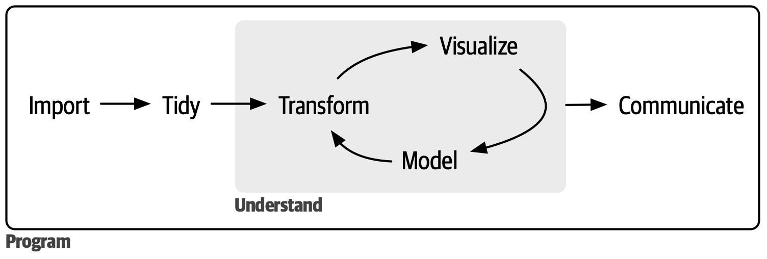 Source: https://r4ds.hadley.nz/intro.html
For now, we’ll take a shortcut and use the skimr package to get a quick overview of the dataset.
skim(stroke_classification)
── Data Summary ────────────────────────
                           Values
Name                       stroke_classification
Number of rows             5110
Number of columns          11
_______________________
Column type frequency:
  character                1
  numeric                  10
________________________
Group variables            None

── Variable type: character ──────────────────────────────────────────────────────────────────────────────────────────
  skim_variable n_missing complete_rate min max empty n_unique whitespace
1 gender                0             1   4   6     0        3          0

── Variable type: numeric ────────────────────────────────────────────────────────────────────────────────────────────
   skim_variable       n_missing complete_rate      mean       sd    p0    p25    p50    p75   p100 hist
 1 pat_id                      0         1     2556.     1475.     1    1278.  2556.  3833.  5110   ▇▇▇▇▇
 2 stroke                      0         1        0.0487    0.215  0       0      0      0      1   ▇▁▁▁▁
 3 age                         0         1       43.2      22.6    0.08   25     45     61     82   ▅▆▇▇▆
 4 hypertension                0         1        0.0975    0.297  0       0      0      0      1   ▇▁▁▁▁
 5 heart_disease               0         1        0.0540    0.226  0       0      0      0      1   ▇▁▁▁▁
 6 work_related_stress         0         1        0.160     0.367  0       0      0      0      1   ▇▁▁▁▂
 7 urban_residence             0         1        0.508     0.500  0       0      1      1      1   ▇▁▁▁▇
 8 avg_glucose_level           0         1      106.       45.3   55.1    77.2   91.9  114.   272.  ▇▃▁▁▁
 9 bmi                       201         0.961   28.9       7.85  10.3    23.5   28.1   33.1   97.6 ▇▇▁▁▁
10 smokes                      0         1        0.630     0.483  0       0      1      1      1   ▅▁▁▁▇
The summary highlights some important issues, the first being the number of missing or NA values in the bmi variable. This matters because we’ll need to decide whether the missingness is systematic or random, and how to handle it later in the workflow.
We also see that gender has three unique levels; for simplicity, we’ll filter to include only phenotypic sexes (male or female). A few other handy manipulations are included in the pipeline, and we’ll save the cleaned output.
stroke_classification_cln <-
  stroke_classification %>%
  as_tibble() %>%
  clean_names() %>%
  filter(gender %in% c("Male", "Female")) %>%
  mutate(across(c(pat_id:gender, hypertension:urban_residence, smokes), as_factor))
One of the key things to assess early on is the class balance of the target variable. If the data are imbalanced, this must be addressed in preprocessing - otherwise, the model will learn to favour the majority class and perform poorly on minority outcomes.
stroke_classification_cln %>%
  ggplot(aes(x = stroke)) +
  geom_bar() +
  labs(title = "Target Variable Class Balance")

Another important consideration is multicollinearity - a situation where two or more predictor variables convey overlapping information or are highly correlated with each other. We should ensure that we identify and, where appropriate, remove highly correlated predictors (typically those with an absolute correlation > 0.8).
stroke_classification_cln %>%
  select(where(is.numeric)) %>%
  filter(!is.na(bmi)) %>%
  cor() %>%
  corrplot(
    method = "color",
    type = "lower",
    col = viridis::viridis(option = "D", n = 10, direction = -1),
    order = "hclust",
    hclust.method = "ward.D",
    tl.cex = 0.75,
    tl.col = "black",
    cl.cex = 0.75
  )
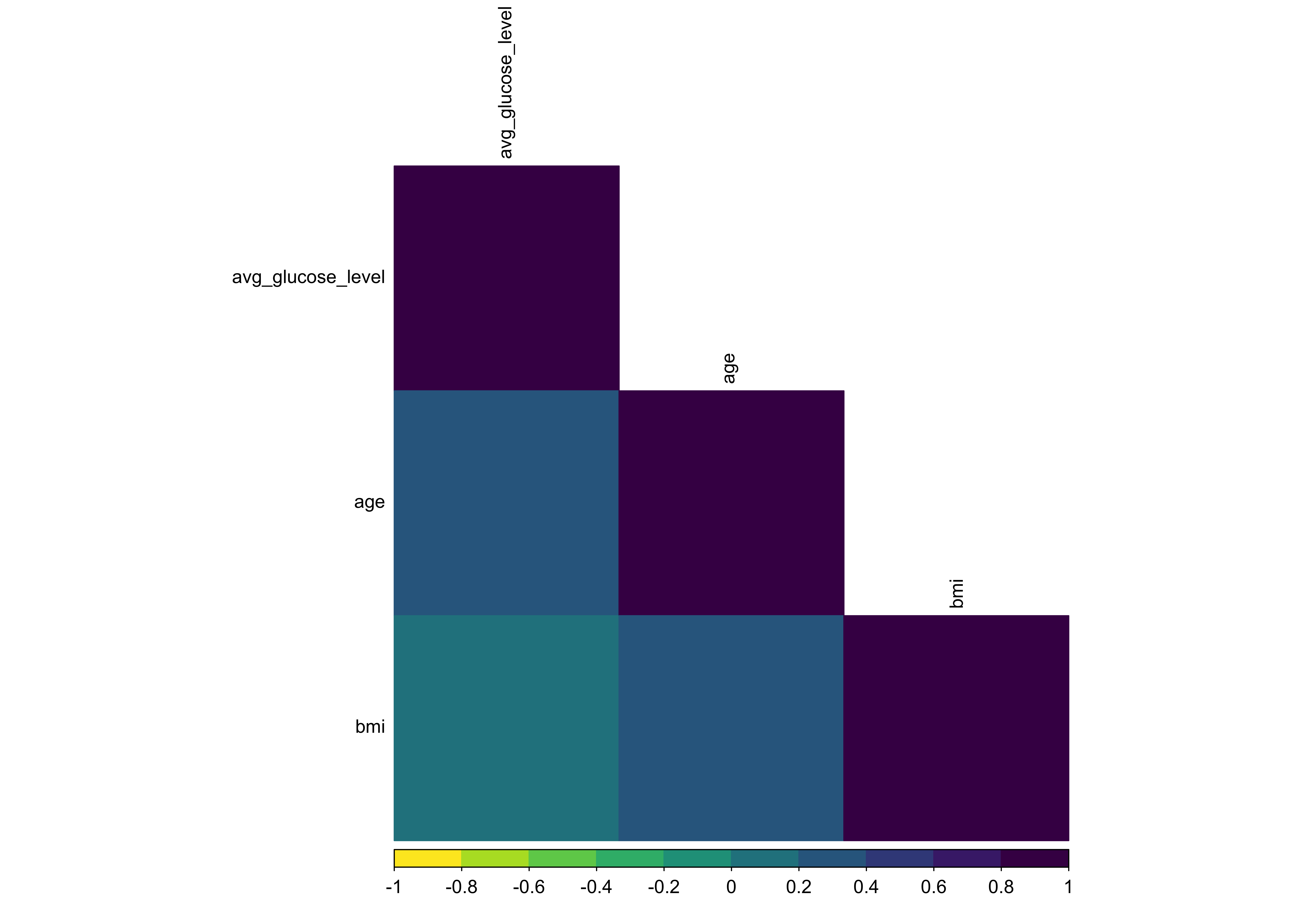
In this case, the correlation plot doesn’t indicate any highly correlated variables that meet the cutoff criteria and which would need to be handled in preprocessing, so we can omit that step later.
At this point, we might create further univariate or multivariate visualisations, but we’ll skip that for brevity. Below are two links to highly recommended YouTube resources for learning more about EDA and its role in the modelling process:
David Robinson - youtube.com/@safe4democracy
Julia Silge - youtube.com/@JuliaSilge
I can’t overstate the importance of EDA as an integral part of modelling - before we choose or fine-tune any algorithm, we need to deeply understand the patterns, relationships, and anomalies in our data. EDA helps us ask better questions, spot potential problems, and guide decisions about how to transform and model the data effectively.
Now that we have explored our data, we are ready to move on to modelling.
Data Splitting
The first step in the modelling workflow proper is to spend our data budget - that is, to split the data into training and testing sets. We’ll use functions from the rsample package, part of the core tidymodels metapackage.
# RNG seed for reproducibility
set.seed(1234)

# data split object
split <-
  initial_split(
    stroke_classification_cln,
    prop = 0.7,
    strata = stroke
  )

# compose training and testing sets
stroke_train <- training(split)
stroke_test <- testing(split)

# sanity check stratification by outcome in splits versus original data
stroke_classification_cln %>%
  count(stroke, name = "count") %>%
  mutate(prop = count / sum(count))

stroke_train %>%
  count(stroke, name = "count") %>%
  mutate(prop = count / sum(count))

stroke_test %>%
  count(stroke, name = "count") %>%
  mutate(prop = count / sum(count))
# original data
# A tibble: 2 × 3
  stroke count   prop
  <fct>  <int>  <dbl>
1 0       4860 0.951
2 1        249 0.0487

# train set
# A tibble: 2 × 3
  stroke count   prop
  <fct>  <int>  <dbl>
1 0       3398 0.950
2 1        178 0.0498

# test set
# A tibble: 2 × 3
  stroke count   prop
  <fct>  <int>  <dbl>
1 0       1462 0.954
2 1         71 0.0463
If we plan to tune model hyperparameters later, we’ll also need to create resamples from the training data (for example, via k-fold cross-validation). We’ll skip this for now but here is where we’ll set up 10-fold CV in the next tutorial where we look at how to tune model hyperparameters.
Preprocessing
Core data preprocessing functions in tidymodels come from the recipes package. As alluded to earlier, all preprocessing steps occur after resampling and are applied independently to the training and testing splits to prevent data leakage. These steps should capture all transformations required by the model - otherwise, new data may break the workflow or yield invalid predictions.
# order here is important!
stroke_rec <-
  recipe(stroke ~ ., data = stroke_train) %>%  # define variable roles
  update_role(pat_id, new_role = "id") %>%     # remove the pat_id variable from predictors
  step_impute_knn(bmi) %>%                     # impute missing BMI using KNN (could tune neighbors here but we won't)
  step_dummy(all_nominal_predictors()) %>%     # dummy encode categorical predictors
  step_normalize(all_numeric_predictors()) %>% # scale the data
  step_smote(stroke)                           # over-sample the minority class

# view preprocessor inputs and operations
stroke_rec
── Recipe ────────────────────────────────────────────────────────────────────────────────────────────────────────────

── Inputs
Number of variables by role
outcome:   1
predictor: 9
id:        1

── Operations
• K-nearest neighbor imputation for: bmi
• Dummy variables from: all_nominal_predictors()
• Centering and scaling for: all_numeric_predictors()
• SMOTE based on: stroke
This step sets up the preprocessor and designates variable roles in the model (predictors, outcomes, or ID labels) but doesn’t yet apply any transformations.
Running prep() on the preprocessor recipe object results in a slightly different output to that shown above; in the latter, only the inputs and operations are shown while running prep() shows training information and confirms the variables used in each step.
prep(stroke_rec)
── Recipe ────────────────────────────────────────────────────────────────────────────────────────────────────────────

── Inputs
Number of variables by role
outcome:   1
predictor: 9
id:        1

── Training information
Training data contained 3576 data points and 138 incomplete rows.

── Operations
• K-nearest neighbor imputation for: bmi | Trained
• Dummy variables from: gender, hypertension, heart_disease, work_related_stress, urban_residence, ... | Trained
• Centering and scaling for: age, avg_glucose_level, bmi, gender_Female, hypertension_X1, ... | Trained
• SMOTE based on: stroke | Trained
If we want to inspect the processed data, we must pass the recipe object to prep() then bake(). Notice that accessing the training data, which is stored in the preprocessor recipe object, requires us to set the new_data argument to NULL. Passing the test data split or the whole data set shows us the result of applying the preprocessor to the respective data set.
# preprocess training split
stroke_rec %>%
  prep() %>%
  bake(new_data = NULL)

# preprocess testing split
stroke_rec %>%
  prep() %>%
  bake(new_data = stroke_test)
One sanity check that’s well worth performing is that the preprocessing step specified to balance the target variable classes (the SMOTE algorithm in this instance) has been applied successfully.
stroke_rec %>%
  prep() %>%
  bake(new_data = NULL) %>%

  ggplot(aes(x = stroke)) +
  geom_bar()
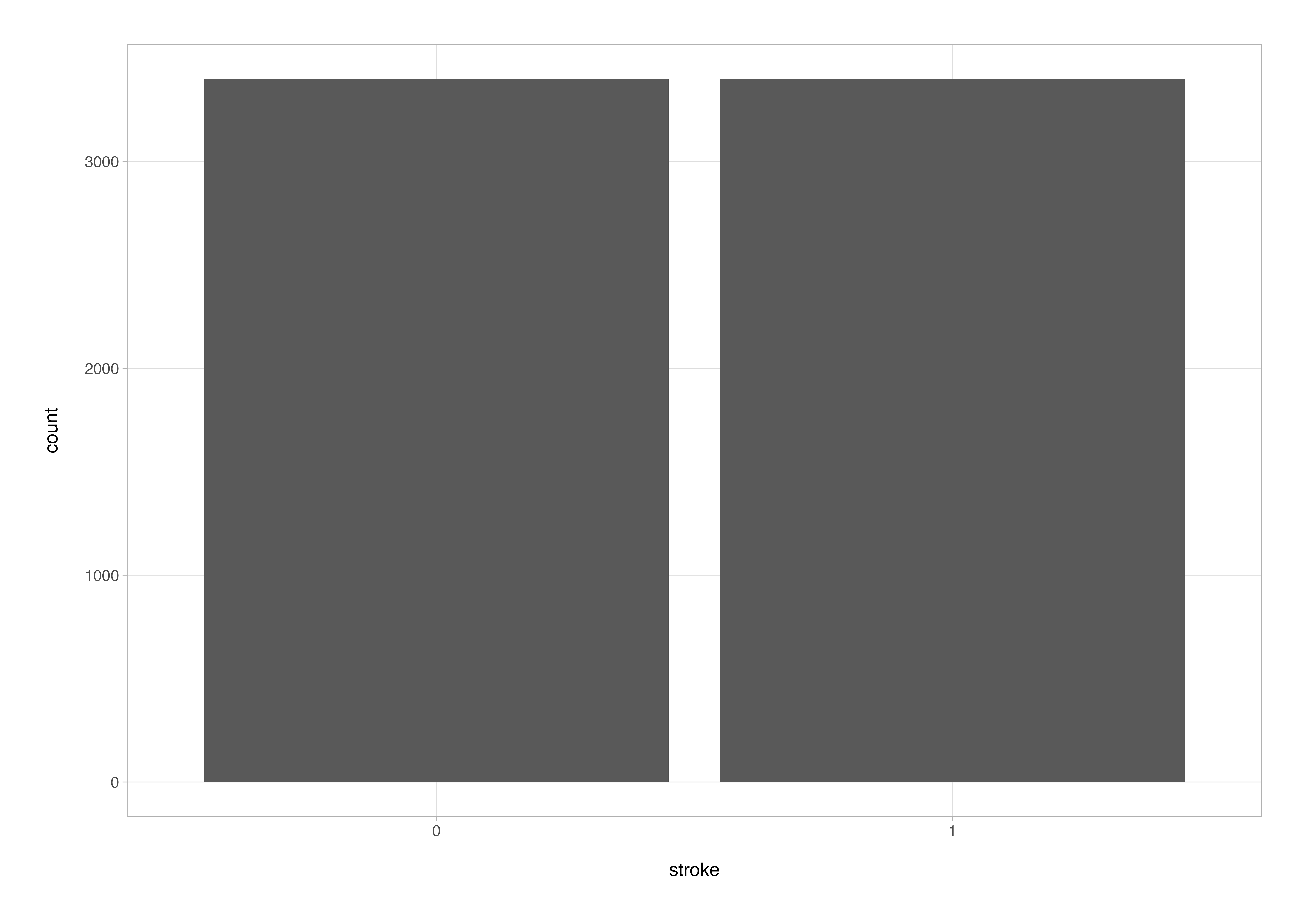
Looks like everything is working as it should be. In case you are wondering how we have suddenly ended up with over 6000 data points for an input data set of 3576 observations (in the training set), that’s SMOTE (Synthetic Minority Over-sampling Technique) in action.
Model Specification
Models in tidymodels are defined using the parsnip package. Its goal is to provide a tidy, unified interface for specifying models, allowing you to swap between algorithms without worrying about the syntax of the underlying packages.
If you’re curious about this, ensure you have the relevant packages installed and then run the following code chunk - it will soon make sense.
# same model type but different package syntax
?ranger::ranger
?randomForest::randomForest

# unified interface
?parsnip::rand_forest
To check which implementations (or engines) are available for a given model type, we can use the show_engines() function.
show_engines("logistic_reg")
Here, we’ll use a generalised linear model for binary outcomes. Since we have a small number of predictors, the glm engine is appropriate.
lr_spec <-
  logistic_reg() %>%
  set_engine("glm") %>%
  set_mode("classification")

lr_spec
Setting the mode in this case isn’t strictly necessary as the only possible value for this model is “classification” but in the name of being declarative I have included it.
Now that we’ve defined both the model and the preprocessor, we can combine them into a single modelling workflow.
Workflow
Workflows make it easy to keep track of which recipe was used to preprocess the data, and which model was used to fit it - both essential for reproducibility.
stroke_wflow <-
  workflow() %>%
  add_model(lr_spec) %>%
  add_recipe(stroke_rec)

stroke_wflow
══ Workflow ══════════════════════════════════════════════════════════════════════════════════════════════════════════
Preprocessor: Recipe
Model: logistic_reg()

── Preprocessor ──────────────────────────────────────────────────────────────────────────────────────────────────────
4 Recipe Steps

• step_impute_knn()
• step_dummy()
• step_normalize()
• step_smote()

── Model ─────────────────────────────────────────────────────────────────────────────────────────────────────────────
Logistic Regression Model Specification (classification)

Computational engine: glm
When you print a workflow object, it provides a concise summary of the full modelling pipeline, showing both the preprocessing and model components. In this example, the preprocessor is a recipe containing the four steps we specified earlier. The model section then shows the model specification, giving a clear overview of how data will flow from raw input to fitted model.
Fit to Training Data
With the workflow ready, we can fit it to the training data.
stroke_fit <-
  stroke_wflow %>%
  fit(data = stroke_train)

stroke_fit
══ Workflow [trained] ════════════════════════════════════════════════════════════════════════════════════════════════
Preprocessor: Recipe
Model: logistic_reg()

── Preprocessor ──────────────────────────────────────────────────────────────────────────────────────────────────────
4 Recipe Steps

• step_impute_knn()
• step_dummy()
• step_normalize()
• step_smote()

── Model ─────────────────────────────────────────────────────────────────────────────────────────────────────────────

Call:  stats::glm(formula = ..y ~ ., family = stats::binomial, data = data)

Coefficients:
           (Intercept)                     age       avg_glucose_level                     bmi
              -1.23213                 1.86866                 0.17456                -0.04219
         gender_Female         hypertension_X1        heart_disease_X1  work_related_stress_X1
              -0.02576                 0.11240                 0.01103                -0.10140
    urban_residence_X1               smokes_X1
               0.05987                 0.15550

Degrees of Freedom: 6795 Total (i.e. Null);  6786 Residual
Null Deviance:      9421
Residual Deviance: 6415   AIC: 6435
The fitted workflow confirms that preprocessing has been applied, and model parameters have been estimated from the processed training data. We can extract the fitted model object from the workflow using extract_fit_parsnip() and then tidy the results using the tidy() function from the broom package for easy interpretation. A couple of extra lines of code neatens the output even further.
stroke_fit %>%
  extract_fit_parsnip() %>%
  tidy() %>%
  filter(term != "(Intercept)") %>%
  arrange(p.value) %>%
  mutate(sig = p.value < 0.05)
# A tibble: 9 × 6
  term                   estimate std.error statistic   p.value sig
  <chr>                     <dbl>     <dbl>     <dbl>     <dbl> <lgl>
1 age                      1.87      0.0533    35.0   5.88e-269 TRUE
2 avg_glucose_level        0.175     0.0289     6.03  1.64e-  9 TRUE
3 smokes_X1                0.155     0.0326     4.77  1.89e-  6 TRUE
4 hypertension_X1          0.112     0.0252     4.46  8.07e-  6 TRUE
5 work_related_stress_X1  -0.101     0.0285    -3.56  3.75e-  4 TRUE
6 urban_residence_X1       0.0599    0.0320     1.87  6.13e-  2 FALSE
7 bmi                     -0.0422    0.0421    -1.00  3.17e-  1 FALSE
8 gender_Female           -0.0258    0.0326    -0.791 4.29e-  1 FALSE
9 heart_disease_X1         0.0110    0.0237     0.465 6.42e-  1 FALSE
At this stage, we could begin to interpret the predictors - but our real concern is model performance: how well does it predict stroke outcomes on unseen data?
Evaluate Model Performance
Now that the model is trained, we can assess its performance using the test set. The augment() function adds the model’s predictions and class probabilities to the test data.
stroke_aug <- augment(stroke_fit, stroke_test)

stroke_aug
# A tibble: 1,533 × 14
   .pred_class .pred_0 .pred_1 pat_id stroke gender   age hypertension heart_disease work_related_stress
   <fct>         <dbl>   <dbl> <fct>  <fct>  <fct>  <dbl> <fct>        <fct>         <fct>
 1 1            0.196    0.804 1      1      Male      67 0            1             0
 2 1            0.0831   0.917 6      1      Male      81 0            0             0
 3 1            0.419    0.581 12     1      Female    61 0            1             0
 4 1            0.0810   0.919 18     1      Male      75 1            0             0
 5 1            0.364    0.636 20     1      Male      57 0            1             0
 6 1            0.228    0.772 29     1      Male      69 0            1             1
 7 1            0.0839   0.916 43     1      Male      82 0            1             0
 8 1            0.378    0.622 44     1      Female    63 0            0             0
 9 1            0.478    0.522 48     1      Female    58 0            0             0
10 0            0.806    0.194 50     1      Female    39 1            0             0
# ℹ 1,523 more rows
# ℹ 4 more variables: urban_residence <fct>, avg_glucose_level <dbl>, bmi <dbl>, smokes <fct>
# ℹ Use `print(n = ...)` to see more rows
From here, we can compute common evaluation metrics using the yardstick package, such as accuracy, sensitivity, and specificity.
For example, accuracy gives us a quick sense of overall performance, while sensitivity and specificity tell us how well the model detects true positives and avoids false alarms, respectively.
# classification metrics
accuracy(stroke_aug, truth = stroke, estimate = .pred_class)
sensitivity(stroke_aug, truth = stroke, estimate = .pred_class)
specificity(stroke_aug, truth = stroke, estimate = .pred_class)
The confusion matrix helps us understand where the model is making errors e.g., false positives (type-I errors) or false negatives (type-II errors).
conf_mat(stroke_aug, truth = stroke, estimate = .pred_class)
           Truth
Prediction     0    1
         0  1079    9
         1   383   62
There’s also an autoplot() method for this so that we can get a nice quick graphical summary.
stroke_aug %>%
  conf_mat(truth = stroke, estimate = .pred_class) %>%
  autoplot(type = "heatmap")
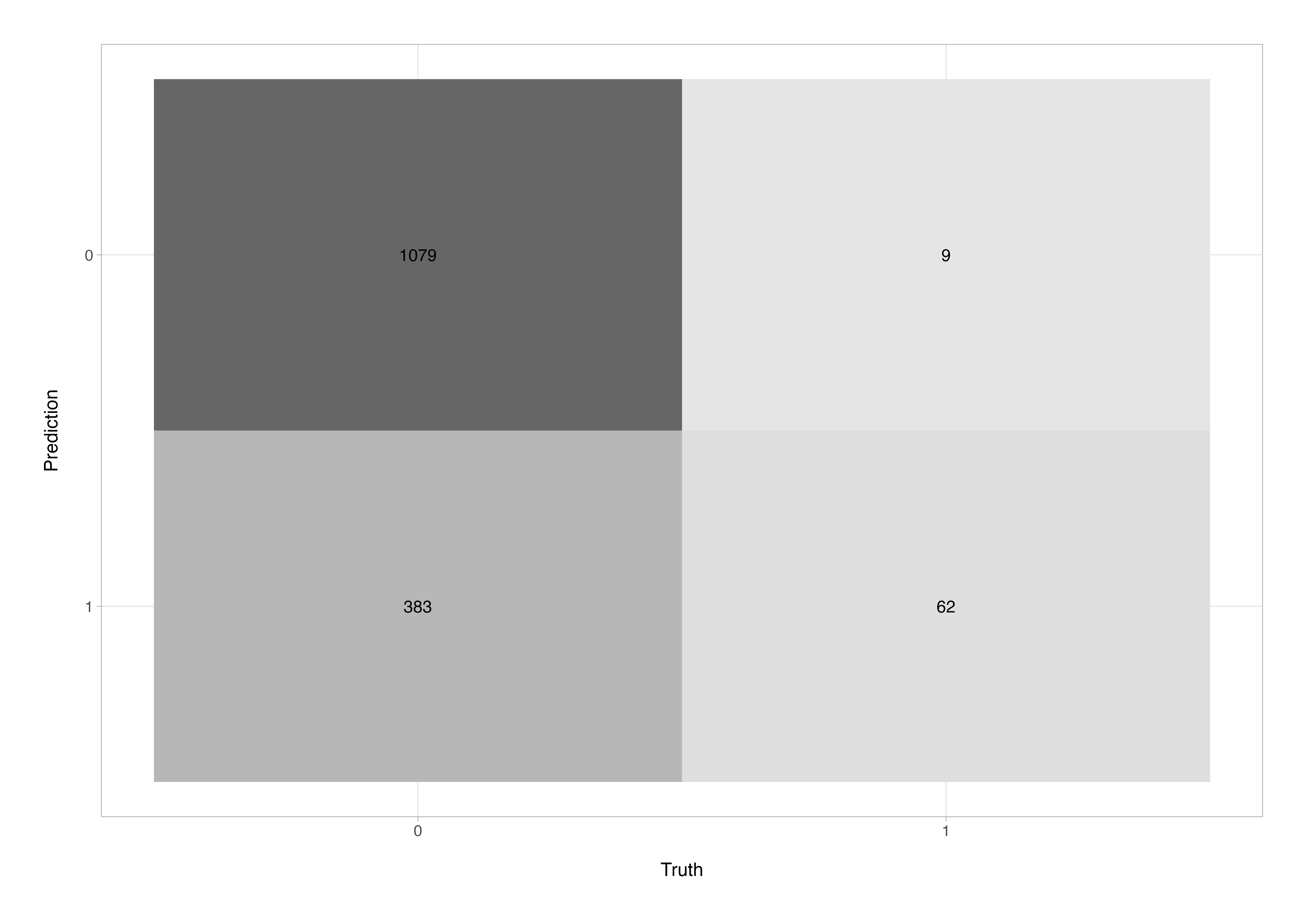
The confusion matrix gives a direct view of how the model performed on the test data. Here, out of 1,533 test cases, 1,079 true negatives (correctly predicted no-stroke) and 62 true positives (correctly predicted stroke) were identified. However, the model also produced 383 false positives - patients incorrectly flagged as at risk - and 9 false negatives or missed stroke cases. While the number of false negatives is reassuringly low (indicating strong sensitivity), the relatively high false-positive rate suggests that the model errs on the side of caution, potentially flagging more patients than necessary. In a clinical screening context, this is often acceptable - prioritising recall (sensitivity) over precision to avoid missing true stroke cases.
When we plot the receiver operating characteristic (ROC) curve, we can see how performance changes across classification thresholds. The area under the curve (AUC) summarises this into a single measure of model discriminative ability.
# roc curve
stroke_aug %>%
  roc_curve(truth = stroke, .pred_0) %>%
  autoplot()

# roc auc value
roc_auc(stroke_aug, truth = stroke, .pred_0)
To plot the ROC curve, the output of the autoplot() function is perfectly servicable but if you love to play with ggplot2 like me, then making a fancier ROC curve that includes the AUC value isn’t too much work 😉
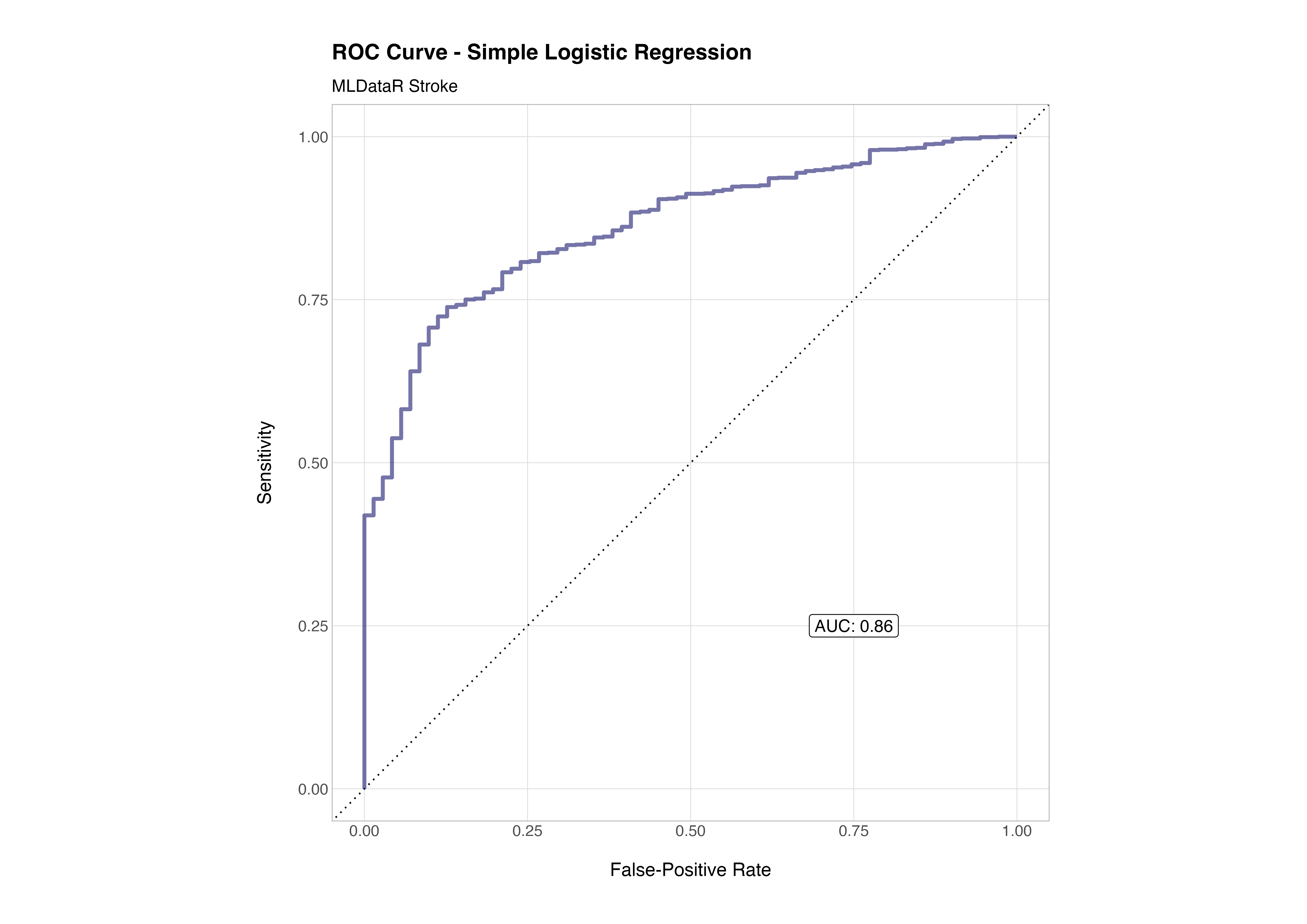
The ROC curve visualises the trade-off between the true positive rate (sensitivity) and the false positive rate (1 - specificity) across different classification thresholds. A model with no discriminative power would follow the diagonal line (AUC = 0.5) which is effectively equivalent to a coin flip, while a perfect classifier would hug the top-left corner (AUC = 1.0).
In this case, the AUC of 0.86 indicates that the model has good discriminative ability - it can correctly distinguish between stroke and non-stroke cases about 86% of the time. That’s a strong performance given the simplicity of the model, minimal feature engineering, and relatively modest preprocessing. It reflects both the informative nature of the underlying features (age, glucose level, hypertension, etc.) and the suitability of logistic regression as a first baseline model for this kind of structured clinical data.
Summary
In this first tutorial, we’ve walked through an end-to-end example of a complete machine learning workflow using the tidymodels framework; from data preparation and preprocessing to model training, evaluation, and interpretation. Along the way, we’ve seen how the components fit together to make modelling both reproducible and elegant. Even with a simple logistic regression model, we achieved an AUC of 0.86 which is proof that well founded and tidy workflows can produce clear, interpretable, and effective results with minimal fuss.
In the next tutorial, we’ll take things a step further by exploring Random Forests, hyperparameter tuning, and feature selection, before looking at how to make our models more interpretable. By the end, you’ll have the tools to move from simple baseline models to robust, fine-tuned predictive pipelines - the tidy way.
See you next time.
Thanks for reading. I hope you enjoyed the article and that it helps you to get a job done more quickly or inspires you to further your data science journey. Please do let me know if there’s anything you want me to cover in future posts.
If this tutorial has helped you, consider supporting the blog on Ko-fi!
Happy Data Analysis!
Disclaimer: All views expressed on this site are exclusively my own and do not represent the opinions of any entity whatsoever with which I have been, am now or will be affiliated.