recall()
In the previous post, we ran through a complete machine learning workflow in R using the tidymodels framework: from exploratory analysis, through data preprocessing, to model training and evaluation, applying a simple logistic regression model to the stroke_classification dataset from the MLDataR package by Gary Hutson.
In this second tutorial, we’ll take the same multivariable binary classification problem - predicting whether someone is at risk of a stroke from lifestyle and health-related variables - but extend the foundations we laid to a more complex model and workflow.
This time, we’ll fit a random forest model and use cross-validation with out-of-sample estimation to iteratively assess performance while tuning model hyperparameters. We’ll then take a brief look at model interpretability - explaining models and their predictions - and close with a short note on feature engineering and selection.
As ever, the first thing we need to do is load our dependencies, define any custom functions (if they aren’t sourced from a file or package), and then load the dataset.
# load packages
library(tidyverse)
library(tidymodels)

library(janitor)
library(MLDataR)
library(skimr)
library(themis)
library(vip)

# custom plot theme
theme_custom <- function() {
  theme_light() +
    theme(
      axis.text = element_text(size = 10),
      axis.title.x = element_text(size = 12, margin = margin(t = 15)),
      axis.title.y = element_text(size = 12, margin = margin(r = 15)),
      panel.grid.minor = element_blank(),
      plot.margin = margin(1, 1, 1, 1, unit = "cm"),
      plot.title = element_text(size = 14, face = "bold", margin = margin(b = 10)),
      strip.background = element_blank(),
      strip.text.x.top = element_text(colour = "black", size = 9, hjust = 0),
      strip.text.y.right = element_text(colour = "black", size = 10, hjust = 0)
    )
}

# set plot theme
theme_set(theme_custom())
To briefly recap, the dataset that we are using stroke_classification contains 5,110 anonymised patient records for 11 variables in total. Of these, five are numeric (continuous health measures such as age or BMI) and six are categorical (binary or factor variables describing demographic and clinical status).
I won’t repeat any exploratory analysis here; for the detailed walkthrough, refer to the previous post. For a quick refresher, we can use skimr::skim() to get a compact overview of the dataset.
# load data
data("stroke_classification")

# dataframe summary
skim(stroke_classification)
── Data Summary ────────────────────────
                           Values
Name                       stroke_classification
Number of rows             5110
Number of columns          11
_______________________
Column type frequency:
  character                1
  numeric                  10
________________________
Group variables            None

── Variable type: character ──────────────────────────────────────────────────────────────────────────────────────────
  skim_variable n_missing complete_rate min max empty n_unique whitespace
1 gender                0             1   4   6     0        3          0

── Variable type: numeric ────────────────────────────────────────────────────────────────────────────────────────────
   skim_variable       n_missing complete_rate      mean       sd    p0    p25    p50    p75   p100 hist
 1 pat_id                      0         1     2556.     1475.     1    1278.  2556.  3833.  5110   ▇▇▇▇▇
 2 stroke                      0         1        0.0487    0.215  0       0      0      0      1   ▇▁▁▁▁
 3 age                         0         1       43.2      22.6    0.08   25     45     61     82   ▅▆▇▇▆
 4 hypertension                0         1        0.0975    0.297  0       0      0      0      1   ▇▁▁▁▁
 5 heart_disease               0         1        0.0540    0.226  0       0      0      0      1   ▇▁▁▁▁
 6 work_related_stress         0         1        0.160     0.367  0       0      0      0      1   ▇▁▁▁▂
 7 urban_residence             0         1        0.508     0.500  0       0      1      1      1   ▇▁▁▁▇
 8 avg_glucose_level           0         1      106.       45.3   55.1    77.2   91.9  114.   272.  ▇▃▁▁▁
 9 bmi                       201         0.961   28.9       7.85  10.3    23.5   28.1   33.1   97.6 ▇▇▁▁▁
10 smokes                      0         1        0.630     0.483  0       0      1      1      1   ▅▁▁▁▇
Recall from last time that the key issues highlighted by this summary overview of the data are missing or NA values in the bmi variable, and more than two levels in the gender variable.
Below are the simple cleaning steps that we used last time to get the data ready for modelling.
stroke_classification_cln <-
  stroke_classification %>%
  as_tibble() %>%
  clean_names() %>%
  filter(gender %in% c("Male", "Female")) %>%
  mutate(across(c(pat_id:gender, hypertension:urban_residence, smokes), as_factor))
We are now ready to begin the modelling process once again.
Data Splitting
As we outlined last time, the first step in the modelling workflow proper is to spend our data budget: create training and testing splits and, if we plan to tune hyperparameters, set up resamples for cross-validation. We’ll use the functions from the rsample package to do this, creating a 70:30 train-test split with stratification to preserve outcome class proportions in each subset.
# RNG seed for reproducibility
set.seed(1234)

# data split object
split <-
  initial_split(
    stroke_classification_cln,
    prop = 0.7,
    strata = stroke
  )

# compose training and testing sets
stroke_train <- training(split)
stroke_test <- testing(split)
As we know we’ll be tuning hyperparameters, we’ll also generate 10-fold cross-validation resamples on the training data. These resamples will be used to estimate performance across different hyperparameter combinations without touching the test set.
# RNG seed for reproducibility
set.seed(1235)

# setup cv folds on training data
stroke_cv <- vfold_cv(stroke_train, v = 10, strata = stroke)
Note that the cross-validation folds are also stratified. This means that, within each iteration, the preprocessor is applied to the nine analysis (training) folds - balancing the outcome classes and allowing the model to learn from these - while the single assessment (testing) fold retains the original class proportions. This approach ensures that the model is trained on balanced data but evaluated on data that reflect the real-world imbalance of the outcome. As a result, the performance metrics calculated across the ten iterations provide a realistic indication of how the final model will behave when fitted to the full training set and applied to unseen data post-deployment.
Preprocessing
Recall that core preprocessing in tidymodels is handled by the recipes package. As we discussed previously, all preprocessing steps should follow data splitting and/or resampling and be applied independently to the training and testing splits to avoid data leakage.
The sequence we use here mirrors the earlier tutorial and reflects what EDA suggested was appropriate for this dataset: addressing missing values in bmi (imputation using k-NN), dummy-encoding of categorical predictors, normalisation of numeric predictors, and balancing of outcome classes in the stroke variable, in this case using SMOTE.
Although tree-based models like random forests aren’t sensitive to feature scaling, we’ll retain the normalisation step here for consistency with our previous workflow and to illustrate how recipes handles preprocessing modularly.
# order here is important!
stroke_rec <-
  recipe(stroke ~ ., data = stroke_train) %>%  # define variable roles
  update_role(pat_id, new_role = "id") %>%     # remove the pat_id variable from predictors
  step_impute_knn(bmi) %>%                     # impute missing BMI using KNN (could tune neighbors here but we won't)
  step_dummy(all_nominal_predictors()) %>%     # dummy encode categorical predictors
  step_normalize(all_numeric_predictors()) %>% # scale the data
  step_smote(stroke)                           # over-sample the minority class

# view preprocessor inputs and operations
stroke_rec
── Recipe ────────────────────────────────────────────────────────────────────────────────────────────────────────────

── Inputs
Number of variables by role
outcome:   1
predictor: 9
id:        1

── Operations
• K-nearest neighbor imputation for: bmi
• Dummy variables from: all_nominal_predictors()
• Centering and scaling for: all_numeric_predictors()
• SMOTE based on: stroke
Recall that defining the recipe sets up roles and steps but doesn’t transform the data until you prep() it, which trains the preprocessor using the training data, and then bake() it. The dataset for preprocessing is passed to the new_data argument of the latter. If you want to inspect the processed training data, bake(new_data = NULL) returns the prepped training set.
Model Setup
We’ll specify a random forest using parsnip. One of the advantages of parsnip is its unified interface: you can swap engines (e.g., ranger, randomForest) without rewriting your modelling code. We’ll use the ranger engine here because it’s fast, well-maintained, and exposes the hyperparameters we’ll tune: mtry, trees, and min_n.
# random forest model spec
rf_spec <-
  rand_forest() %>%
  set_mode("classification") %>%
  set_engine("ranger") %>%
  set_args(
    mtry = tune(),
    trees = tune(),
    min_n = tune(),
  )
I personally prefer this modular, declarative way of setting the model mode, engine, and hyperparameter arguments - tagging those we intend to tune using the tune() function. This approach keeps the model definition clean and consistent with the tidy modelling philosophy. However, you can also specify everything directly within rand_forest() itself, as shown below.
rf_spec <-
  rand_forest(
    mode = "classification",
    engine = "ranger",
    mtry = tune(),
    trees = tune(),
    min_n = tune()
  )

rf_spec
Random Forest Model Specification (classification)

Main Arguments:
  mtry = tune()
  trees = tune()
  min_n = tune()

Computational engine: ranger
The advantage of the modular approach is that it offers far greater flexibility: you can update or replace the model specification, swap engines, or adjust hyperparameters without redefining the entire model object. This makes experimentation and iteration much smoother and more reproducible, especially during model comparison or tuning.
Workflow
We’ll combine the recipe and model into a single workflow. This keeps preprocessing and modelling tightly coupled and reproducible, ensuring that transformations are always applied consistently before fitting.
rf_wflow <-
  workflow() %>%
  add_recipe(stroke_rec) %>%
  add_model(rf_spec)

rf_wflow
══ Workflow ══════════════════════════════════════════════════════════════════════════════════════════════════════════
Preprocessor: Recipe
Model: rand_forest()

── Preprocessor ──────────────────────────────────────────────────────────────────────────────────────────────────────
4 Recipe Steps

• step_impute_knn()
• step_dummy()
• step_normalize()
• step_smote()

── Model ─────────────────────────────────────────────────────────────────────────────────────────────────────────────
Random Forest Model Specification (classification)

Main Arguments:
  mtry = tune()
  trees = tune()
  min_n = tune()

Computational engine: ranger
What we have seen so far has not been so different from the previous tutorial; other than setting up cross-validation folds and specifying a different model with tuneable hyperparameters. Here’s where we go through the looking glass…
Tuning Hyperparameters
In the first tutorial, we fit our workflow once to the training set and then evaluated on the testing set. Rather than fitting once on the full training set, we’ll tune hyperparameters by fitting across the cross-validation folds that we setup earlier.
To do this, we first need to define a grid of plausible values for mtry, trees, and min_n.
# define hyperparameter tuning permutations
tuning_grid <-
  expand_grid(
    mtry = seq(1, 6, 2),
    trees = seq(500, 2000, 500),
    min_n = seq(0, 100, 20)
  )
Here, we’re constructing it manually using expand_grid() from tidyr, but the tidymodels ecosystem also provides the dials package, which is purpose-built for this task; it provides helper functions for generating structured tuning grids, all beginning with grid_ . These include regular grids (grid_regular()), random grids (grid_random()), and space-filling grids such as Latin hypercube designs (grid_latin_hypercube()). These functions automatically generate combinations of parameter values based on their defined ranges and types, allowing systematic exploration of the hyperparameter space in balance with computational efficiency.
To establish a combination of hyperparameters that is optimal for our specific data set and modelling task, we must evaluate each combination using metrics such as sensitivity, specificity, and ROC AUC. We can define these as a metric_set object either pre-defined in our environment or passed directly to the metrics argument of tune_grid(). In our case we will create an object so we can compute the same evaluation metrics when we assess model performance on unseen data later on.
# RNG seed for reproducibility
set.seed(1236)

# register a parallel back-end
future::plan(future::multisession(), workers = parallel::detectCores() - 1)

# model evaluation metric set
eval_metrics <- metric_set(sens, spec, roc_auc)

# fit to resamples and perform tuning
rf_tuning <-
  rf_wflow %>%
  tune_grid(
    resamples = stroke_cv,
    grid = tuning_grid,
    metrics = eval_metrics,
    control = control_resamples(save_pred = TRUE)
  )
Parallelisation here helps speed up the grid search on multi-core machines. When you consider that the regular grid we defined contains 72 hyperparameter combinations, and with 10-fold cross-validation, we are fitting 720 individual models: one for each combination–fold pairing. This is why parallel processing is essential for tuning non-trivial models efficiently.
I have a MacBook Pro M2 and this step using 7 CPU cores and 16GB RAM takes about 10 minutes. So you can either run this and wait, perhaps have a cup of tea in the interim, or you can download the tuning result object from here and load it as follows, ensuring you specify the correct path to the file as you see fit:
rf_tuning <- read_rds(file = "rf_tuning.rds")
Once you have the tuning result in your environment, we can see how the model performance varies according to different permutations of the tuning parameters - either by manually extracting and plotting the metrics, or more conveniently using autoplot().
# plot tuning results
autoplot(rf_tuning)
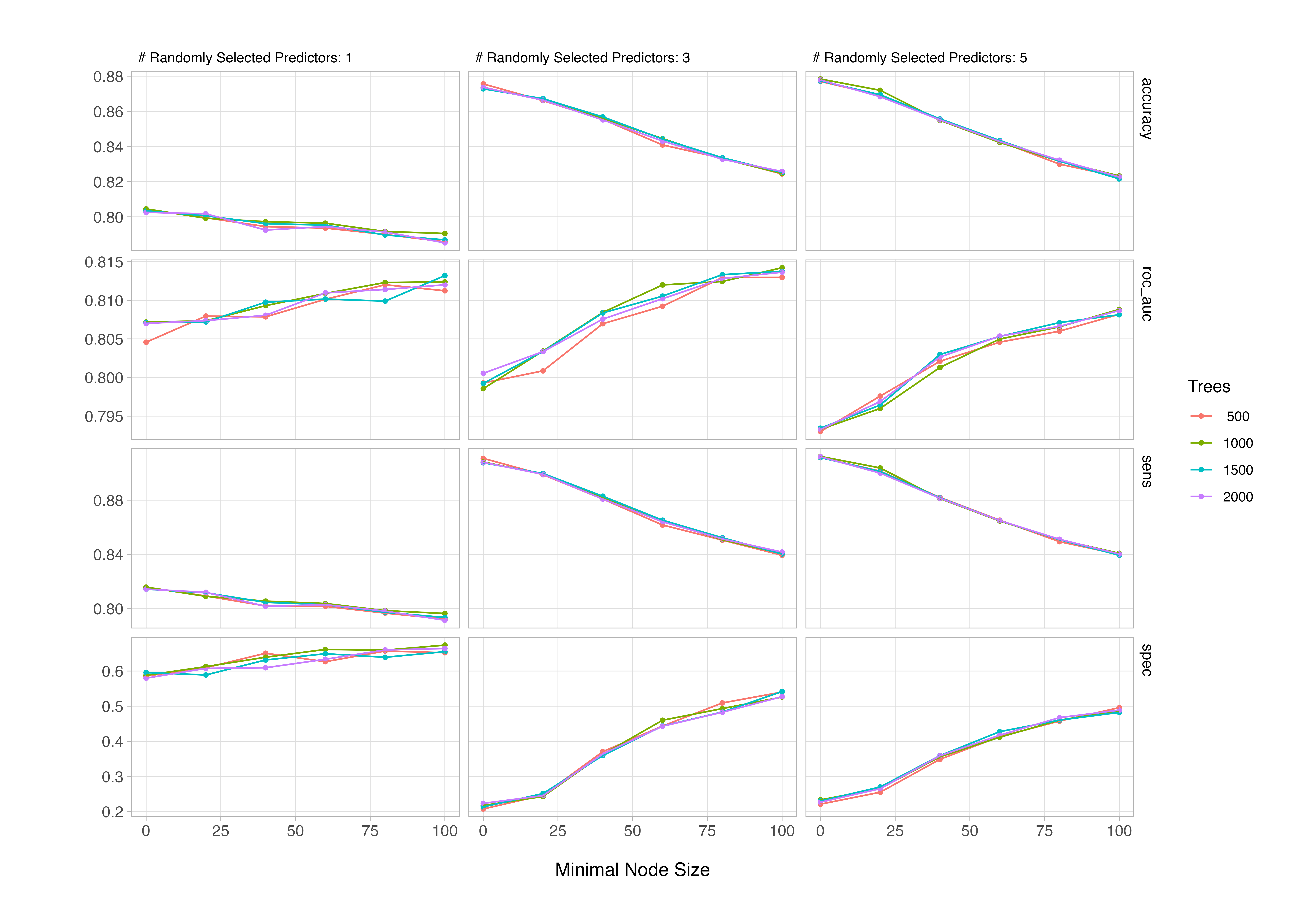
From the plot, we can see that the number of trees has little impact on performance; generally, once the number of trees exceeds a few hundred, gains tend to flatten out and additional trees primarily reduce variance rather than bias. The ROC AUC curves show that model performance improves as the minimal node size min_n increases up to around 75, suggesting that slightly larger terminal nodes help reduce overfitting in this dataset. The best results (highest ROC AUC around 0.86) occur when mtry, or the number of predictors randomly sampled at each split, is relatively small (around 3). This indicates that introducing more randomness between trees improves generalisation.
In practice, this pattern is typical for moderately correlated predictor sets: too few variables limit learning, while too many makes trees more alike and reduces ensemble diversity.
Finalising the Model
Even if you’ve been doing this for a while and can eyeball reasonable hyperparameter settings, best guesses aren’t good science. The whole point of tuning is to be systematic and reproducible. Fortunately, tidymodels provides a suite of functions to help you identify and extract the best-performing combination of hyperparameters based on a chosen metric. That choice of metric is critical. Here, we’ll use ROC AUC, which offers a balanced view of performance by integrating both sensitivity and specificity, an appropriate trade-off for a healthcare classification problem like stroke prediction.
show_best(rf_tuning, metric = "roc_auc", n = 5)
# A tibble: 5 × 9
   mtry trees min_n .metric .estimator  mean     n std_err .config
  <dbl> <dbl> <dbl> <chr>   <chr>      <dbl> <int>   <dbl> <chr>
1     3  1000   100 roc_auc binary     0.814    10 0.00458 pre0_mod48_post0
2     3  1500   100 roc_auc binary     0.814    10 0.00479 pre0_mod54_post0
3     3  2000   100 roc_auc binary     0.814    10 0.00459 pre0_mod60_post0
4     3  1500    80 roc_auc binary     0.813    10 0.00525 pre0_mod53_post0
5     1  1500   100 roc_auc binary     0.813    10 0.00486 pre0_mod24_post0
Once we’ve identified the best hyperparameter combination (e.g., by highest mean ROC AUC across folds), we finalise the workflow with those values.
# select best model with respect to chosen metric
rf_best <- select_best(rf_tuning, metric = "roc_auc")

# finalise the model specification post-tuning
rf_tuned <- finalize_model(rf_spec, parameters = rf_best)

# finalise workflow by updating with the tuned model
rf_final <-
  rf_wflow %>%
  update_model(rf_tuned)

rf_final
══ Workflow ══════════════════════════════════════════════════════════════════════════════════════════════════════════
Preprocessor: Recipe
Model: rand_forest()

── Preprocessor ──────────────────────────────────────────────────────────────────────────────────────────────────────
4 Recipe Steps

• step_impute_knn()
• step_dummy()
• step_normalize()
• step_smote()

── Model ─────────────────────────────────────────────────────────────────────────────────────────────────────────────
Random Forest Model Specification (classification)

Main Arguments:
  mtry = 3
  trees = 1000
  min_n = 100

Computational engine: ranger
We could alternatively finalise the workflow by splicing-in the optimal model hyperparameters in one step as shown below.
# update the workflow with the final model spec
rf_final <- finalize_workflow(rf_wflow, parameters = rf_best)
The reason for having the tuned model object available rather than finalising the workflow in this manner will be immediately obvious in the section on variable importance measures; essentially, we’d have to extract it from the workflow there anyway, so might as well keep it separate here.
Final Fit to Test Data
The tune package has a convenient function last_fit() that enables us to retrain on the entire training set and evaluate once on the test set. This gives us an honest estimate of out-of-sample performance after tuning.
# RNG seed for reproducibility
set.seed(1237)

# fit to train and evaluate on test
rf_final %>%
  last_fit(split = split, metrics = eval_metrics) %>%
  collect_metrics()
# A tibble: 3 × 4
  .metric .estimator .estimate .config
  <chr>   <chr>          <dbl> <chr>
1 sens    binary         0.856 pre0_mod0_post0
2 spec    binary         0.535 pre0_mod0_post0
3 roc_auc binary         0.823 pre0_mod0_post0
As convenient as this is, it’s also useful to compute the model’s performance on the training data. Doing so lets us assess how well the model generalises and whether it may have overfit the training data. However, we shouldn’t rely on performance estimates from the cross-validation folds used during hyperparameter tuning as those are inherently optimistic due to optimisation bias.
The simplest way to evaluate performance on the training data is to augment() the pre-processed training set with predictions from the fitted workflow and then apply our eval_metrics object (which is also a function 😱) to calculate all chosen metrics simultaneously.
# fit to train and evaluate on train
rf_final %>%
  fit(stroke_train) %>%
  augment(stroke_train) %>%
  eval_metrics(truth = stroke, estimate = .pred_class, .pred_0)
# A tibble: 3 × 3
  .metric .estimator .estimate
  <chr>   <chr>          <dbl>
1 sens    binary         0.866
2 spec    binary         0.831
3 roc_auc binary         0.938
You’ll notice that the performance on the training data looks noticeably stronger than on the last_fit() results from the held-out test set. That’s perfectly normal. The first set of metrics comes from fitting the model directly to the full training data, which means the model has already “seen” those examples and can adapt closely to them, while the last_fit() output reflects performance on completely unseen data.
The drop in ROC AUC from 0.94 to 0.82 and the sharper fall in specificity show that the model doesn’t generalise quite as well as it fits the training data, a reminder that even robust algorithms like random forests can overfit if left unchecked. This is exactly why we reserve a test set: it gives us a realistic picture of how the model will perform in the wild. That said, an AUC of 0.82 is still a solid result.
Model Interpretability: Variable Importance
Random forests don’t provide coefficients or p-values like our logistic regression model from last week, so how do we reason about which variables drive predictions? One practical route is permutation importance.
We can refit the tuned model on the fully pre-processed data (excluding IDs), compute permutation importance by setting a ranger engine-specific argument (importance) and visualise the resulting scores. This isn’t causal, but it does provide a useful ranking of features based on their contribution to predictive performance in this model.
# extract entire prepped data set and remove id variables
rf_vip_data <-
  stroke_rec %>%
  prep() %>%
  bake(new_data = NULL) %>%
  select(!pat_id)

# refit the model one time to prepped data set
rf_vip <-
  rf_tuned %>%
  set_args(importance = "permutation") %>%
  fit(stroke ~ ., data = rf_vip_data) %>%
  vi()
# A tibble: 9 × 2
  Variable               Importance
  <chr>                       <dbl>
1 age                       0.180
2 bmi                       0.0548
3 avg_glucose_level         0.0495
4 smokes_X1                 0.0326
5 urban_residence_X1        0.0291
6 gender_Female             0.0209
7 work_related_stress_X1    0.0162
8 hypertension_X1           0.0146
9 heart_disease_X1          0.00867
We can then plot these results as an ordered horizontal bar chart. In this case, the feature set is small enough that visualisation adds little beyond the table itself, but with larger or more complex models, visualising variable importance can be an invaluable interpretability aid, helping to quickly identify which predictors drive model behaviour.
# plot the variable importance metrics
rf_vip %>%
  mutate(
    Variable = Variable %>%
      str_remove("_.\\d") %>%
      str_replace_all("_", " ") %>%
      str_to_title() %>%
      str_replace("Bmi", "BMI") %>%
      fct_reorder(Importance)
  ) %>%

  ggplot(aes(x = Importance, y = Variable)) +
  geom_col() +
  labs(y = NULL)
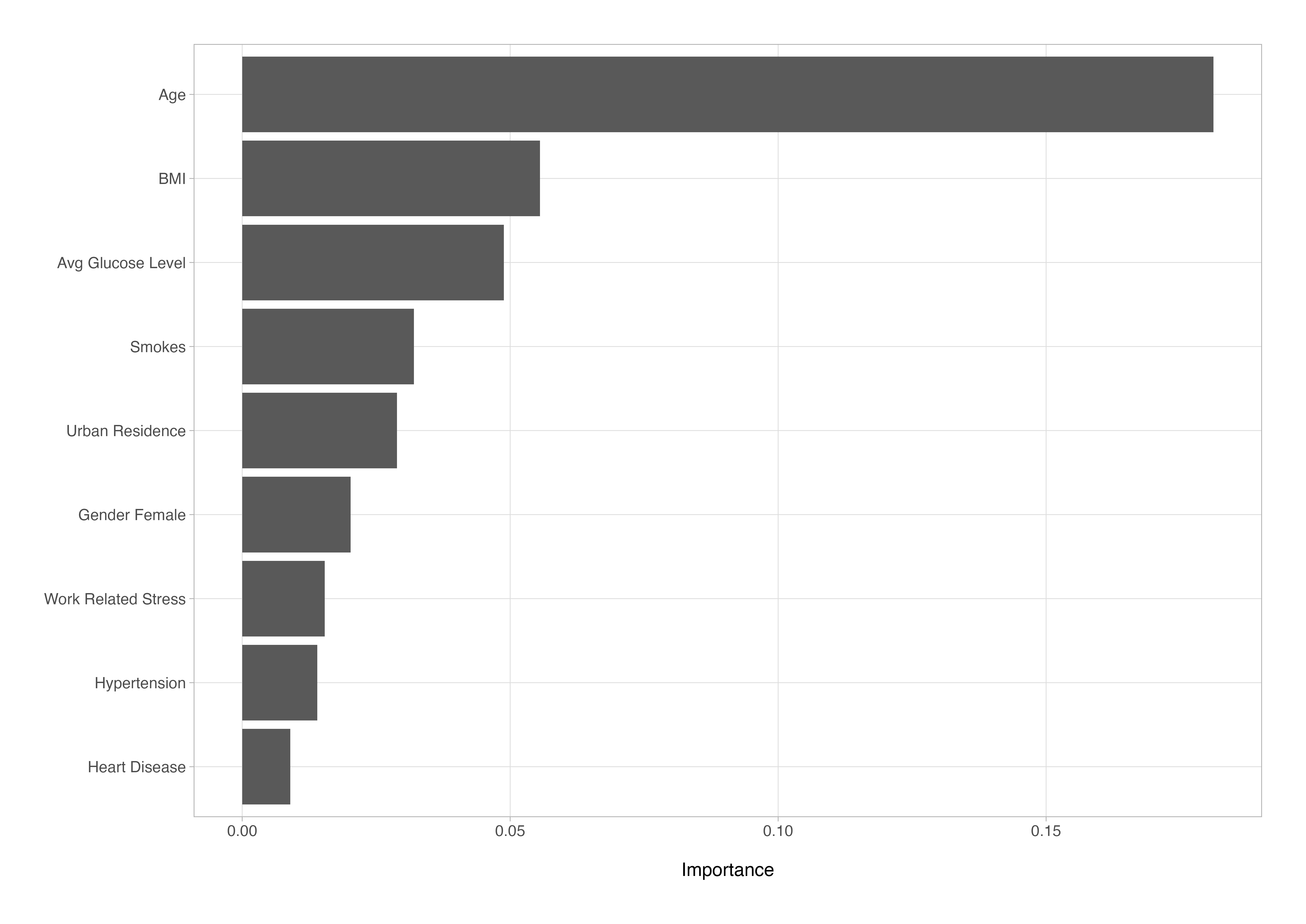
The permutation importance scores represent how much model performance decreases when each feature’s values are randomly shuffled. In effect, they indicate how strongly the model depends on each variable for accurate prediction - higher values suggest greater influence, though they’re not literal percentage contributions.
Permutation importance offers a global view of which features influence the model most overall. We could complement this with local interpretability methods, such as SHAP or LIME, to explain individual predictions. In all honesty, I could write an entire post or series on model interpretability as it’s such a detailed topic in its own right…perhaps I will 🤔
A Quick Look at Feature Selection
Feature selection is another one of those topics that entire books have been written on, so I’ll keep it brief here, but it’s worth pausing to show just how influential it can be.
Although it’s often approached algorithmically, feature selection doesn’t have to be. In practice, we can draw on domain knowledge, use regularised models, or rely on measures such as permutation importance to simplify the feature set and improve generalisability.
For instance, if we said that we don’t think that those features with permutation importance values lower than 0.05 were contributing meaningfully to the model, we could remove them in the recipe and benchmark the difference. The aim isn’t to chase tiny gains, but to build simpler, more robust models that generalise well and are easier to explain.
Here’s a quick minimal workflow to allow us to investigate this.
# define variables to remove based on feature importance
vars_to_rm <-
  rf_vip %>%
  mutate(Importance = round(Importance, digits = 3)) %>%
  filter(Importance < 0.05) %>%
  pull(Variable) %>%
  str_remove("_X1|_Female")

# updated recipe - remove unwanted features
stroke_rec_updt <-
  recipe(stroke ~ ., data = stroke_train) %>%
  update_role(pat_id, new_role = "id") %>%
  step_rm(all_of(vars_to_rm)) %>%
  step_impute_knn(bmi) %>%
  step_dummy(all_nominal_predictors()) %>%
  step_normalize(all_numeric_predictors()) %>%
  step_smote(stroke)

# updated workflow with new preprocessing recipe
rf_wflow_updt <-
  rf_wflow %>%
  update_recipe(stroke_rec_updt)

# retune hyperparameters
set.seed(1238)

rf_tuning_updt <-
  rf_wflow_updt %>%
  tune_grid(
    resamples = stroke_cv,
    grid = tuning_grid,
    metrics = eval_metrics,
    control = control_resamples(save_pred = TRUE)
  )
To save you the time running this, I have made the rf_tuning_updt object available to download from here.
# update the workflow with the final model spec
rf_updt_tuned <- finalize_workflow(rf_wflow_updt, parameters = select_best(rf_tuning_updt, metric = "roc_auc"))

# train set performance
rf_updt_tuned %>%
  fit(stroke_train) %>%
  augment(stroke_train) %>%
  eval_metrics(truth = stroke, estimate = .pred_class, .pred_0)
# A tibble: 3 × 3
  .metric .estimator .estimate
  <chr>   <chr>          <dbl>
1 sens    binary         0.849
2 spec    binary         0.854
3 roc_auc binary         0.945
# test set performance
rf_updt_tuned %>%
  last_fit(split = split, metrics = eval_metrics) %>%
  collect_metrics()
# A tibble: 3 × 4
  .metric .estimator .estimate .config
  <chr>   <chr>          <dbl> <chr>
1 sens    binary         0.829 pre0_mod0_post0
2 spec    binary         0.563 pre0_mod0_post0
3 roc_auc binary         0.814 pre0_mod0_post0
The simplified model that is trained on a reduced set of predictors trades a little raw performance for parsimony.
On the training data it looks very strong, but on the unseen test set those metrics are reduced. The drops that we observe, especially in specificity and AUC, signals some overfitting relative to the training fit, but it’s not catastrophic and is consistent not only with what we expect when we simplify the feature space but with what we saw on the full data set. Compared to the full model (sens = 0.86, spec = 0.54, AUC = 0.82), the reduced version offers a modest gain in specificity (+0.02) with a small cost in sensitivity (−0.03) and AUC (−0.01).
In other words, you get a leaner, easier-to-explain model with broadly similar discriminative ability. This is very useful if interpretability and maintainability matter as much as squeezing out the last point of ROC AUC.
summarise()
Over these two tutorials, we’ve built a complete machine learning workflow in tidymodels, going from data exploration and preprocessing through model tuning, evaluation, and interpretation. Along the way, we’ve seen how the tidy modelling framework encourages a declarative, modular approach to analysis: each step is explicit, reproducible, and easily adapted to new models or datasets.
In this second part, we stepped beyond simple logistic regression to explore random forests, introducing cross-validation, hyperparameter tuning, and variable importance as practical extensions of the tidy modelling grammar. We also saw that complexity doesn’t always equal performance. Careful feature selection and sound validation strategy can produce models that are not only competitive but easier to interpret and deploy.
This closes out the introductory series, but there’s much more to come. In future posts, I’ll take a closer look at questions that often arise once you’re comfortable with the basics: how to choose the right model for a particular problem, more advanced resampling strategies and how data characteristics influence resampling strategy, and how to balance interpretability with predictive performance.
Until then, happy modelling.
Thanks for reading. I hope you enjoyed the article and that it helps you to get a job done more quickly or inspires you to further your data science journey. Please do let me know if there’s anything you want me to cover in future posts.
If this tutorial has helped you, consider supporting the blog on Ko-fi!
Happy Data Analysis!
Disclaimer: All views expressed on this site are exclusively my own and do not represent the opinions of any entity whatsoever with which I have been, am now or will be affiliated.