The Tidyverse
Like many, I got my start in R doing everything “the hard way” in the base language. However, as my interest and aspirations shifted from learning enough R for basic bioinformatics towards becoming a qualified full-time data professional and instructor, my habits also shifted away from base R towards the glorious tidyverse ecosystem.
The tidyverse is a collection of R packages for data science that use common data structures and share an underlying design philosophy and grammar.
The paradigm shift that my R usage underwent happened for a few reasons, paramount amongst which was the realisation that tidyverse packages just make data science so much easier and faster to both do and learn. I can still swing with the best of them when it comes to base R, don’t get me wrong, but I don’t. Why go to the effort?
Consider the following example:
# example 1
my_data[my_data$variable_1 == "Some String", ]

# example 2
filter(my_data, variable_1 == "Some String")
Now tell me what you think each code snippet does and which one is a) most intuitive and b) easiest to implement in a real-world setting without getting errors? Both lines of code in fact do the exact same thing. The first example is base R syntax while the second is tidyverse syntax. Now imagine doing much more complex tasks using each syntax type. You get my point, right?
Given that I have just started a YouTube channel and the direction I will be moving in over the course of 2023 will be towards more advanced data analysis screencasts that heavily feature both the tidyverse and tidymodels (the equivalent of tidyverse for machine learning in R), I thought a quick primer video to demo some fundamental tidyverse functions would be appropriate.
So here it is, my inaugural screencast tutorial. I hope you enjoy it 🍿
TL;DW
In this tutorial, I use a data set for Billboard Hot 100 songs taken from the TidyTuesday project and cover the basics of piping, the workhorse data frame subsetting functions select() and filter() from the dplyr package, how to extract distinct and arrange rows of a data frame for specific combinations of variables, and how to relocate and rename variables. I also quickly showcase a simple example of plotting with the ggplot2 package using the example data frame resulting from the tutorial and produce a graph showing that Eminem got beat by a girl!!
Linked Resources
dplyr cheatsheet
ggplot cheatsheet
Tutorial Code
The code block below will load the packages required to prepare the data and run all the code featured in the tutorial. Defining and applying a customised plotting theme isn’t mandatory, but it does make plots look nice 😉
# load libraries
library("tidyverse")
library("lubridate")
library("magrittr")

# custom plot theme
theme_custom <- function() {
  theme_light() +
    theme(
      axis.text = element_text(size = 10),
      axis.title.x = element_text(size = 12, margin = margin(15, 0, 0, 0)),
      axis.title.y = element_text(size = 12, margin = margin(0, 15, 0, 0)),
      panel.grid.minor = element_blank(),
      plot.margin = margin(1, 1, 1, 1, unit = "cm"),
      plot.title = element_text(size = 14, face = "bold", margin = margin(0, 0, 10, 0))
    )
}

# set plot theme
theme_set(theme_custom())
The data set used in the tutorial is from the TidyTuesday project, which is a weekly data project aimed at users of the R ecosystem and is run by the R for Data Science Online Learning Community.
The data set contains the Billboard Hot 100 songs of the week for each week dating back to 1st January 1966 and can be found here.
The “Billboard Hot 100” is the music industry standard record chart in the United States for songs, published weekly by Billboard magazine. Chart rankings are based on sales (physical and digital), radio play, and online streaming in the United States.
df <- read_csv('https://raw.githubusercontent.com/rfordatascience/tidytuesday/master/data/2021/2021-09-14/billboard.csv')
The code chunk below will construct the data frame “billboard_top_100” that I use throughout the remainder of the tutorial. Don’t worry too much about making sense of it at this point, just run it.
# basic data filtration and cleaning
billboard_top_100 <- df %>%
  select(
    date = week_id,
    rank = week_position,
    song,
    artist = performer,
    previous_week_position,
    peak_position,
    weeks_on_chart
  ) %>%
  filter(
    mdy(date) %>%
      year() %>%
      is_greater_than(2010)
  ) %>%
  arrange(
    mdy(date) %>%
      year(),
    mdy(date) %>%
      month(),
    mdy(date) %>%
      day(),
    rank
  )
1. pipe operator
The first concept we will cover is something that you will see used with all tidyverse packages a lot; the %>% or pipe operator used for piping.
Piping is where everything that comes before the pipe is evaluated and (by default) passed in as the first argument of the function that comes after the pipe.
Piping is useful for chaining series of functions together to keep code readable and to minimise the number of variables stored in memory.
# print the first 10 data frame rows to the console using base R syntax
head(billboard_top_100, n = 10)

# print the first 10 data frame rows to the console using piping
billboard_top_100 %>%
  head(n = 10)

# explicitly specify the pipe output position
10 %>%
  head(billboard_top_100, n = .)
2. select
The select() function selects the columns that you specify using a concise mini-language that makes it easy to refer to variables based on their name, index number, properties, or using a series of helper functions.
# positively select using column names
billboard_top_100 %>%
  select(date, rank, song, artist, weeks_on_chart)

# positively select using column names using operators to aid selection
billboard_top_100 %>%
  select(date:artist, weeks_on_chart)

# rename columns inside select()
billboard_top_100 %>%
  select(date, rank, song, artist, "weeks_on_board" = weeks_on_chart)

# negatively select (drop) using column names
billboard_top_100 %>%
  select(!c(previous_week_position, peak_position))
The examples shown are just a very limited number relative to the many possible ways of selecting variables using the select() function. Refer to the help documents using help("select") or ?dplyr::select. Alternatively, consult the dplyr cheatsheet for more information.
3. mutate
The mutate() function adds new variables to a data frame and preserves existing ones. Here, we add a new column called “collab” that indicates whether a song was a collaboration between artists by testing for the pattern “Featuring” within each character string within the “artist” column.
billboard_top_100 %>%
  mutate(collab = str_detect(artist, pattern = "Featuring"))
4. relocate
The relocate() function can be used to change column positions. It uses the same syntax as select() in order to make it easy to move blocks of columns at once.
Let’s relocate the “collab” column we created in the previous example so that it is located immediately after the “artist” column.
billboard_top_100 %>%
  mutate(collab = str_detect(artist, pattern = "Featuring")) %>%
  relocate(collab, .after = artist)
5. filter
The filter() function is used to subset a data frame, retaining all rows that meet one or more conditions.
From the previous example, we know that the str_detect() function returns a logical vector, so we can use it with filter() in order to extract rows from the data frame.
# filter based on a single condition
billboard_top_100 %>%
  filter(str_detect(artist, pattern = "Featuring"))

# multiple conditions: both must evaluate to TRUE for row to be returned
billboard_top_100 %>%
  filter(
    str_detect(artist, pattern = "Featuring"),
    weeks_on_chart >= 20
  )

# multiple conditions: either can evaluate to TRUE for row to be returned
billboard_top_100 %>%
  filter(artist == "Eminem" | artist == "P!nk")
These are just a couple of simple examples of the filter function. As with select(), the filter() function can be used with a large number of operators and functions in order to construct expressions that evaluate to Boolean values. As with select(), it would be advisable to read the help() documentation and the dplyr cheatsheet to really get a handle on how to use it effectively.
6. distinct
The distint() function extracts only unique/distinct rows from a data frame.
In this example, we can filter the data to songs for only the artists Eminem and P!nk and return the distinct combinations of artists and songs in our filtered data frame.
billboard_top_100 %>%
  filter(artist == "Eminem" | artist == "P!nk") %>%
  distinct(artist, song)
7. arrange
The arrange() function orders the rows of a data frame by the values of selected columns.
If we wanted to order data frame that we composed in the previous example according to artist in alphabetical order then we could do so using the arrange() function.
billboard_top_100 %>%
  filter(artist == "Eminem" | artist == "P!nk") %>%
  distinct(artist, song) %>%
  arrange(artist)
To arrange in descending order, we have to wrap each variable in the desc() function
billboard_top_100 %>%
  filter(artist == "Eminem" | artist == "P!nk") %>%
  distinct(artist, song) %>%
  arrange(desc(artist))
We could also order artist and then their songs in alphabetical order
billboard_top_100 %>%
  filter(artist == "Eminem" | artist == "P!nk") %>%
  distinct(artist, song) %>%
  arrange(artist, song)
It is possible to use almost any combination of variables and the desc() function to get data frame rows in the exact order desired.
8. group_by
Most data operations are done on groups defined by variables and the group_by() function takes a data frame and groups it so that operations are performed “by group”.
billboard_top_100 %>%
  filter(artist == "Eminem" | artist == "P!nk") %>%
  group_by(artist, song)
Running the above in applies grouping to the data but doesn’t do anything meaningful in isolation; we must pass these groups to another function which will operate on them.
9. summarise
The summarise() function creates a new data frame containing one (or more) rows for each combination of grouping variables, and one column for each grouping variable and summary statistic specified.
billboard_top_100 %>%
  filter(artist == "Eminem" | artist == "P!nk") %>%
  group_by(artist, song) %>%
  summarise(total_weeks = n())
In this case, applying summarise() to the groups formed from “artist” and “song” variables allows us to calculate the total number of rows for each group, which is equivalent to the number of entries in the Billboard Hot 100 for each song by a specific artist i.e., it gives us the total number of weeks each song was on the chart.
There are many other summary functions that can be used along with summarise() to compute summaries of our data. Some of these are detailed in the help documentation and the dplyr cheat sheet. It is also possible to use user-defined functions to apply bespoke summaries to data.
10. ggplot
Plotting in the tidyverse is taken care of by the excellent ggplot2 package. Let’s make a quick plot for the summarised data we have been working on.
# data wrangling code
billboard_top_100 %>%
  filter(artist == "Eminem" | artist == "P!nk") %>%
  group_by(artist, song) %>%
  summarise(total_weeks = n()) %>%
  mutate(song = fct_reorder(song, total_weeks)) %>%

  # plotting code
  ggplot(aes(x = total_weeks, y = song, fill = artist)) +
  geom_col() +
  scale_fill_manual(values = c("khaki", "hotpink")) +
  labs(
    title = "Eminem vs P!nk",
    subtitle = "Time Spent by Songs on the Billboard Top 100 (2010 - 2021)",
    x = "Weeks",
    y = NULL,
    fill = "Artist"
  )
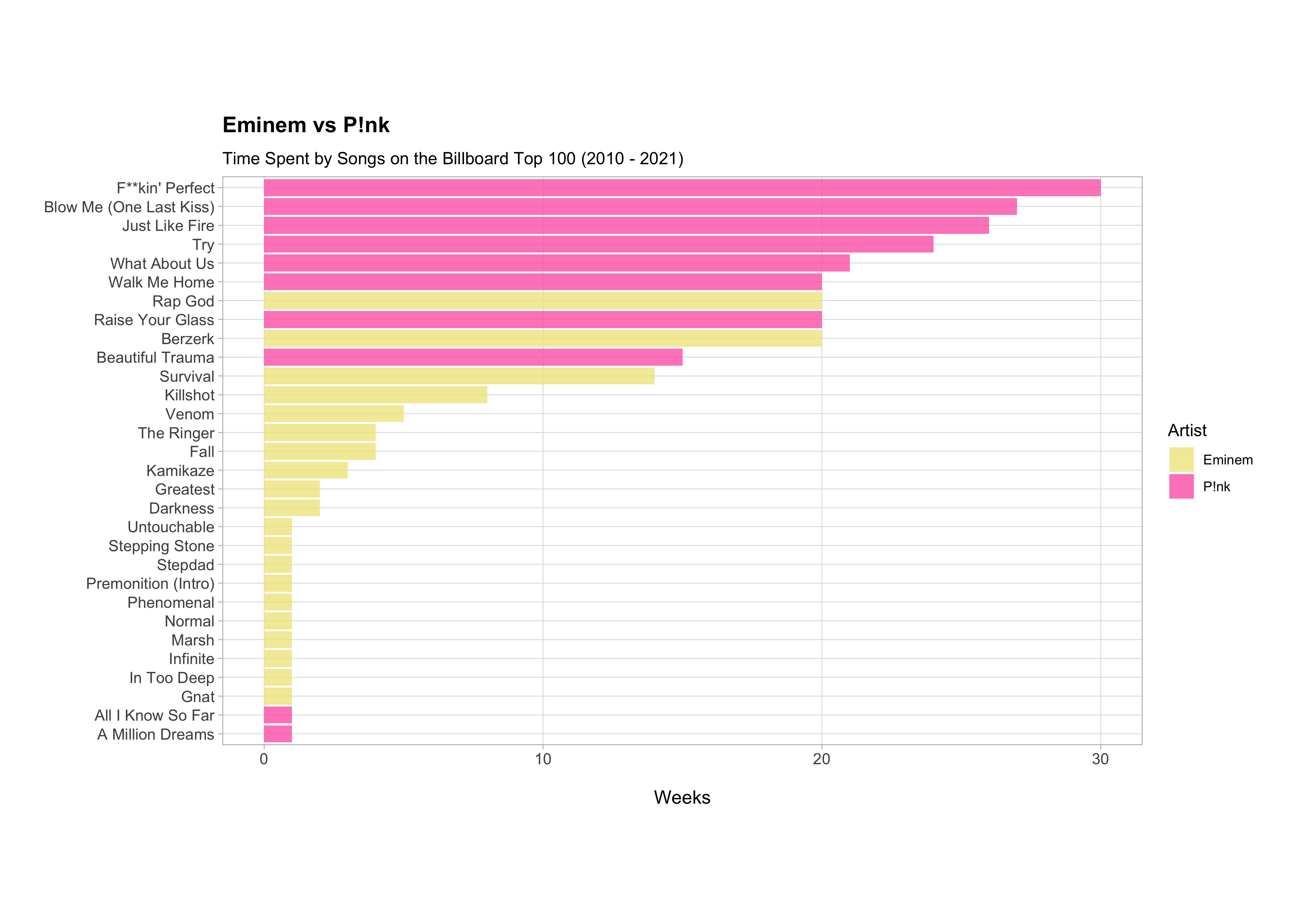
According to this graph, P!nk had fewer songs that entered the Billboard Hot 100 between 2010 and 2021 compared to Eminem, half the number in fact (10 songs compared to 20 songs), but her songs spent much more time on the chart; 80% of her songs were on the chart for 10 weeks or more compared to only 15% of Eminem songs.
This is a really simple demonstration of the capability of ggplot() function but plotting in ggplot2 is really a topic that requires a series of tutorials in it’s own right. A short while back, I wrote a couple of posts on my blog providing an introduction to the theory of ggplot2; here are the links to part 1 and part 2. Keep an eye out for the follow-up ggplot2 tutorials that I will be putting out in the future.
Summary()
Hopefully this tutorial has demonstrated the potential and power of the R tidyverse for data analysis; we have been able to go from raw data to insight using just a few simple examples of tidyverse functions. The foundational functions shown here form the basis for many data wrangling and data exploration tasks in R.
I might do a series featuring some more functions and advanced use-cases at some point in the future, and I have a bunch of handy tidyverse tricks that I will definitely be doing a tutorial on at some point.
Catch you next time!
View Session Info
## ─ Session info ───────────────────────────────────────────────────────────────
##  setting  value
##  version  R version 4.2.1 (2022-06-23)
##  os       macOS Big Sur ... 10.16
##  system   x86_64, darwin17.0
##  ui       X11
##  language (EN)
##  collate  en_US.UTF-8
##  ctype    en_US.UTF-8
##  tz       Europe/London
##  date     2023-01-10
##  pandoc   2.17.1.1 @ /Applications/RStudio.app/Contents/MacOS/quarto/bin/ (via rmarkdown)
##
## ─ Packages ───────────────────────────────────────────────────────────────────
##  package     * version date (UTC) lib source
##  cli           3.4.1   2022-09-23 [1] CRAN (R 4.2.0)
##  digest        0.6.31  2022-12-11 [1] CRAN (R 4.2.0)
##  evaluate      0.19    2022-12-13 [1] CRAN (R 4.2.1)
##  fastmap       1.1.0   2021-01-25 [1] CRAN (R 4.2.0)
##  glue          1.6.2   2022-02-24 [1] CRAN (R 4.2.0)
##  htmltools     0.5.4   2022-12-07 [1] CRAN (R 4.2.0)
##  knitr         1.41    2022-11-18 [1] CRAN (R 4.2.0)
##  lifecycle     1.0.3   2022-10-07 [1] CRAN (R 4.2.1)
##  magrittr      2.0.3   2022-03-30 [1] CRAN (R 4.2.0)
##  rlang         1.0.6   2022-09-24 [1] CRAN (R 4.2.0)
##  rmarkdown     2.18    2022-11-09 [1] CRAN (R 4.2.0)
##  rstudioapi    0.14    2022-08-22 [1] CRAN (R 4.2.0)
##  sessioninfo   1.2.2   2021-12-06 [1] CRAN (R 4.2.0)
##  stringi       1.7.8   2022-07-11 [1] CRAN (R 4.2.0)
##  stringr       1.5.0   2022-12-02 [1] CRAN (R 4.2.0)
##  vctrs         0.5.1   2022-11-16 [1] CRAN (R 4.2.0)
##  xfun          0.35    2022-11-16 [1] CRAN (R 4.2.0)
##  yaml          2.3.6   2022-10-18 [1] CRAN (R 4.2.0)
##
##  [1] /Library/Frameworks/R.framework/Versions/4.2/Resources/library
##
## ──────────────────────────────────────────────────────────────────────────────
Thanks for reading. I hope you enjoyed the article and that it helps you to get a job done more quickly or inspires you to further your data science journey. Please do let me know if there’s anything you want me to cover in future posts.
Happy Data Analysis!
Disclaimer: All views expressed on this site are exclusively my own and do not represent the opinions of any entity whatsoever with which I have been, am now or will be affiliated.