Previously on Data Fundamentals…
In my last post in this Data Fundamentals series I spoke about the importance of understanding data types. I also alluded to the somewhat related topic of this post: levels of measurement.
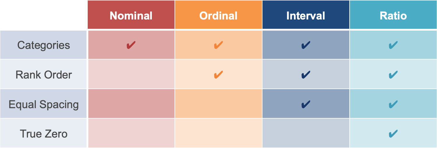
Levels of measurement, also called scales of measurement, describe the accuracy with which the values of a variable are recorded. There are four levels of measurement: nominal, ordinal, interval and ratio. These are organised hierarchically from lowest (nominal) to highest (ratio) in order of accuracy and cumulative complexity.
Those of you that bothered to read my post on data types might have noticed that “nominal” and “ordinal” are also categorical data types. Indeed, they are. These labels indicate both the type of data and their relative level of measurement. The other two data types, discrete and continuous numerical data, can be measured at either the interval or ratio level. Correct identification of both the data type and the level of measurement of variables within a data set are of equal importance. Let’s take a closer look.
Levels of Measurement
The nominal level of measurement is the least accurate and complex level. The word nominal means “existing in name only”. Nominal data can therefore be labelled as belonging to one of the mutually exclusive groups that exist within a variable but there is no implicit order between categories. A good example of this is modes of transport. The data recorded for this variable can be sorted into categories (e.g. car, bus, train, tram, bike, etc.) but we can’t say that one mode of transport is better or worse than the other, despite what Mr Toad or Lucky Jackson would have you believe.
The ordinal level of measurement is the next level in terms of accuracy and complexity. Ordinal data can be classified into categories within a variable as well as having a rank order. However, it is not possible to infer anything about the intervals between the rankings. For example, although you can rank the top 3 Formula 1 Drivers, this scale itself does not tell you how close or far apart they are in terms of number of wins, simply who is the best. Just for reference, the best Formula 1 Driver is Lewis Hamilton. You see now why there’s a disclaimer in the footer and no comments section. 😉
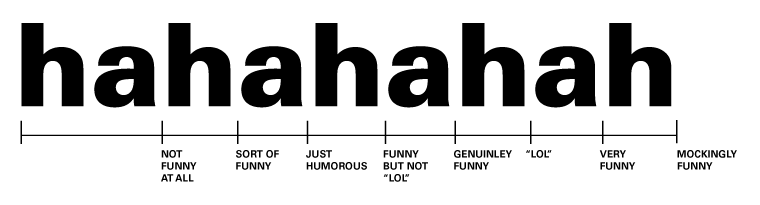 Comic Value: Rate Your Response to My Bad Jokes on an Ordinal Scale
The interval level is the third most accurate and complex of the levels of measurement. Interval data are measured on a numerical scale that has equal distances (intervals) between adjacent, inherently ordered values. There is no true zero on an interval scale; zero is an arbitrary point, not a complete absence of the variable. Temperature on the Celsius scale is an example of a variable measured on the interval scale. The difference between any two adjacent temperatures is constant (1°C) and the intervals are ranked in order of numerical value, but 0°C isn’t the lowest possible temperature and doesn’t mean an absolute absence of thermal energy.
The ratio level is the most accurate and complex of the levels of measurement. Like interval data, ratio data are measured on an ordered numerical scale that has equal distances between adjacent data points. Unlike interval data, however, ratio scales do possess a true zero. Temperature on the Kelvin scale is an example of a ratio variable. On the Kelvin temperature scale, the difference between any two adjacent temperatures is constant and the intervals are ranked in order of numerical value but 0K does mean an absolute lack of thermal energy.
 Levels of Measurement
A couple of important (and perhaps obvious) things to note:
-
Interval and ratio variables can be of either a discrete or continuous type i.e. expressed as integers (e.g. 10°C, 284K etc.) or fractional numbers (10.10°C, 283.25K etc.). Put another way, discrete or continuous numerical data types can be measured at either the interval or ratio level.
-
It is only possible to calculate ratios with data recorded on a ratio scale. For example, although 20°C is half as many °C as 40°C, it isn’t half as hot! This is because temperature measured in Celsius is recorded at the interval level, lacks true zero, and is therefore only relative; there isn’t half the amount of thermal energy. On the other hand, 20K is half as hot as 40K; the difference is absolute because there is a true zero at the starting point of the Kelvin scale. Got that? 0K.
The TL;DR
Values recorded at the ratio level can be categorised, ordered, have equal intervals and take on a true zero. The presence of a true zero makes it possible to multiply, divide or take the square root of values. Recording data on a ratio level is preferable to other levels because it is the most accurate.
Why Are They Important?
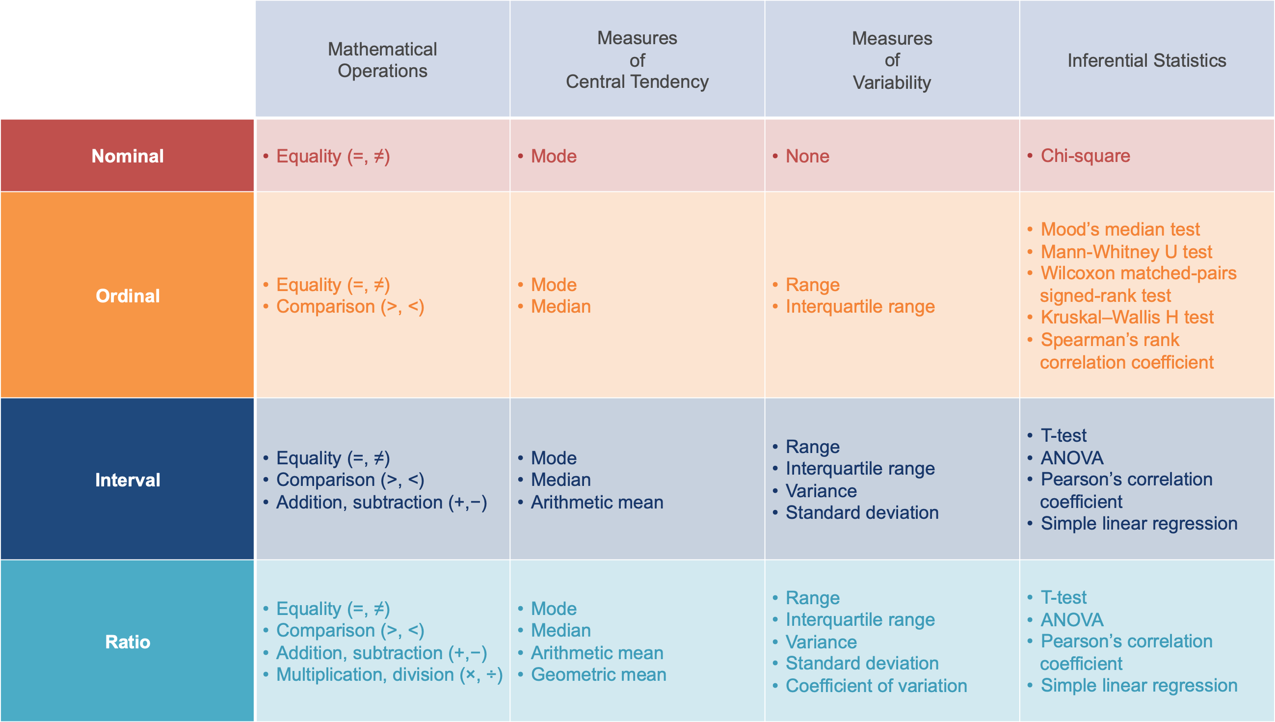
In short; like the type of data, the level of measurement at which a variable is recorded prescribes both the descriptive statistics that can be used to summarise and describe the data, and the inferential statistical methods that can be performed on those data to support or refute a specific hypothesis. The table below contains examples of some of the descriptive and inferential statistics that can be applied at each level of measurement based on the mathematical operations that are appropriate for each level.
 Click to Zoom
In many cases, variables can be measured at more than one different level. It is therefore important when designing an experiment to decide upon the appropriate or desired level of measurement prior to undertaking data collection. Similarly, when undertaking data analysis, it is important to consider whether conversion of one or more variables to lower levels of measurement is necessary, useful or appropriate. Given that all mathematical operations and measures used at lower levels can be applied to variables recorded at higher levels, this decision often comes down to how well a given summary statistic or graphical modelling technique assists development of narrative.
If you have made it this far and looked at that table thinking “I don’t maths or stats, what are all these words?” then don’t panic; my next post in this series will be about commonly used descriptive statistics. In future posts I will cover how to calculate descriptive statistics in R and how to use them effectively during data analysis. I will also write posts on inferential statistics and their practical use cases. Watch this space.
Thanks for reading. I hope you enjoyed the article and that it helps you to get a job done more quickly or inspires you to further your data science journey. Please do let me know if there’s anything you want me to cover in future posts.
Happy Data Analysis!
Disclaimer: All views expressed on this site are exclusively my own and do not represent the opinions of any entity whatsoever with which I have been, am now or will be affiliated.