There is a peculiar and deeply ingrained ritual in biological research, one that has unfortunately become so ubiquitous that it is rarely questioned. A researcher measures something inherently continuous (e.g., gene expression, protein abundance, immune infiltration, tumour mutational burden, etc.) and then, almost reflexively, they divide it into two groups: high versus low. Usually above versus below the median but sometimes upper quartile or another quantile versus the remainder. A Kaplan-Meier curve is plotted. A log-rank p-value is generated. A figure is produced that appears authoritative, clinical, and interpretable. And, more often than not, a claim is made that the biomarker is “prognostic”.
Here we go again…🤦🏻
In that moment of apparent clarity, something important has been lost. What began as a rich, continuous biological signal is abruptly forced into a binary structure - reduced to a crude step function. Nuance has been sacrificed for convenience. And to make matters worse, the statistical assumptions underpinning those decisions are frequently not interrogated.
This post is about reductivist practices; about the routine dichotomisation of continuous variables in survival analysis; and about why these quietly undermine the very principles of precision medicine that biomarker-centric research claims to advance.
The Seductive Simplicity of the Median Split
Without question, the Kaplan-Meier estimator is one of the most widely used and respected tools in clinical research. It is robust to censoring, visually intuitive, and deeply embedded within translational research culture. Its graphical output resembles the kinds of survival trajectories clinicians encounter in real world practice. It communicates risk over time in a way that feels tangible and grounded. It is, in many ways, an elegant statistical solution to a complicated problem.
However, Kaplan-Meier curves require categorical groupings. They do not operate directly on continuous predictors. Continuous biomarkers, by definition, lack inherent thresholds. They exist along a continuum. But because Kaplan-Meier analysis demands groups, researchers routinely manufacture them.
The median split has become the default solution. It is attractive precisely because it appears neutral, defensible and transferable. By splitting at the median, group sizes are balanced. No one can accuse the analyst of favouring one direction over another. The threshold seems objective because it emerges directly from the data distribution. It avoids the appearance of cherry-picking. It simplifies interpretation. It produces two clean survival curves that are easy to compare and easy to publish (unfortunately so, more often than not).
This apparent neutrality is deceptive. A median split is not biologically informed nor statistically optimal. It is simply convenient. Dichotomising (and by extension polychotomising) a continuous variable discards information, reduces statistical power, and implicitly assumes that the relationship between biomarker level and outcome behaves as a step function. It not only forces a model in which risk changes abruptly at a single arbitrary value but also makes the estimated effect entirely dependent on where the cut happens to fall within that dataset.
In what might be one of the most understated conclusions in biostatistics, Altman, Royston and Sauerbrei1 described the practice of arbitrary stratification nearly two decades ago as “a bad idea”. Indeed. But while their critique was grounded in solid statistical principles, the warning remains widely ignored in contemporary biomarker research. The persistence of median splits reflects the powerful cultural appeal of simple binary narratives in medical science.
A Concrete Example: ERBB2 in METABRIC
The consequences of this practice are real and demonstrable. In the METABRIC breast cancer discovery cohort of 995 patients, applying a median split to expression levels of the ERBB2 gene yields a log-rank p-value of 0.51. Under the conventional logic of survival analysis, this result would be interpreted as evidence that ERBB2 expression does not significantly stratify relapse-free survival in that cohort. The (incorrect) conclusion that logically follows: the biomarker is uninformative.
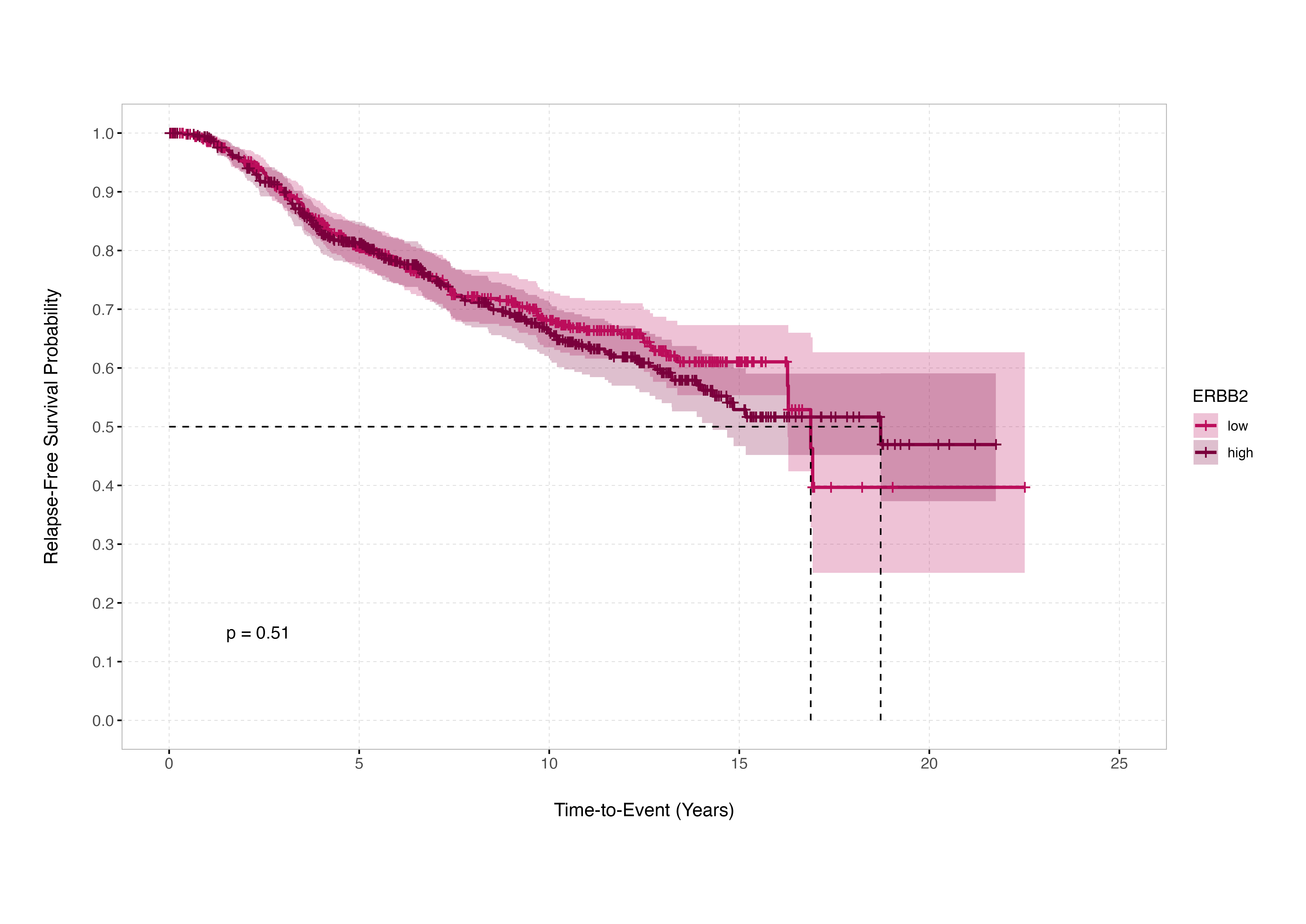 Source:
Naeemaee, R. et al. (2026) Innovations in Biomarker Stratification for Precision Oncology
Source:
Naeemaee, R. et al. (2026) Innovations in Biomarker Stratification for Precision Oncology
This collapses under closer inspection. When every possible dichotomisation point across the ordered ERBB2 expression range is properly evaluated, 344 distinct cut points show statistically significant associations with survival outcome. Crucially, none of these significant thresholds lie at or near the median. The median split fails not because ERBB2 lacks prognostic value, but because the biological effect is not aligned with the 50th percentile: the chosen threshold suppresses the signal.
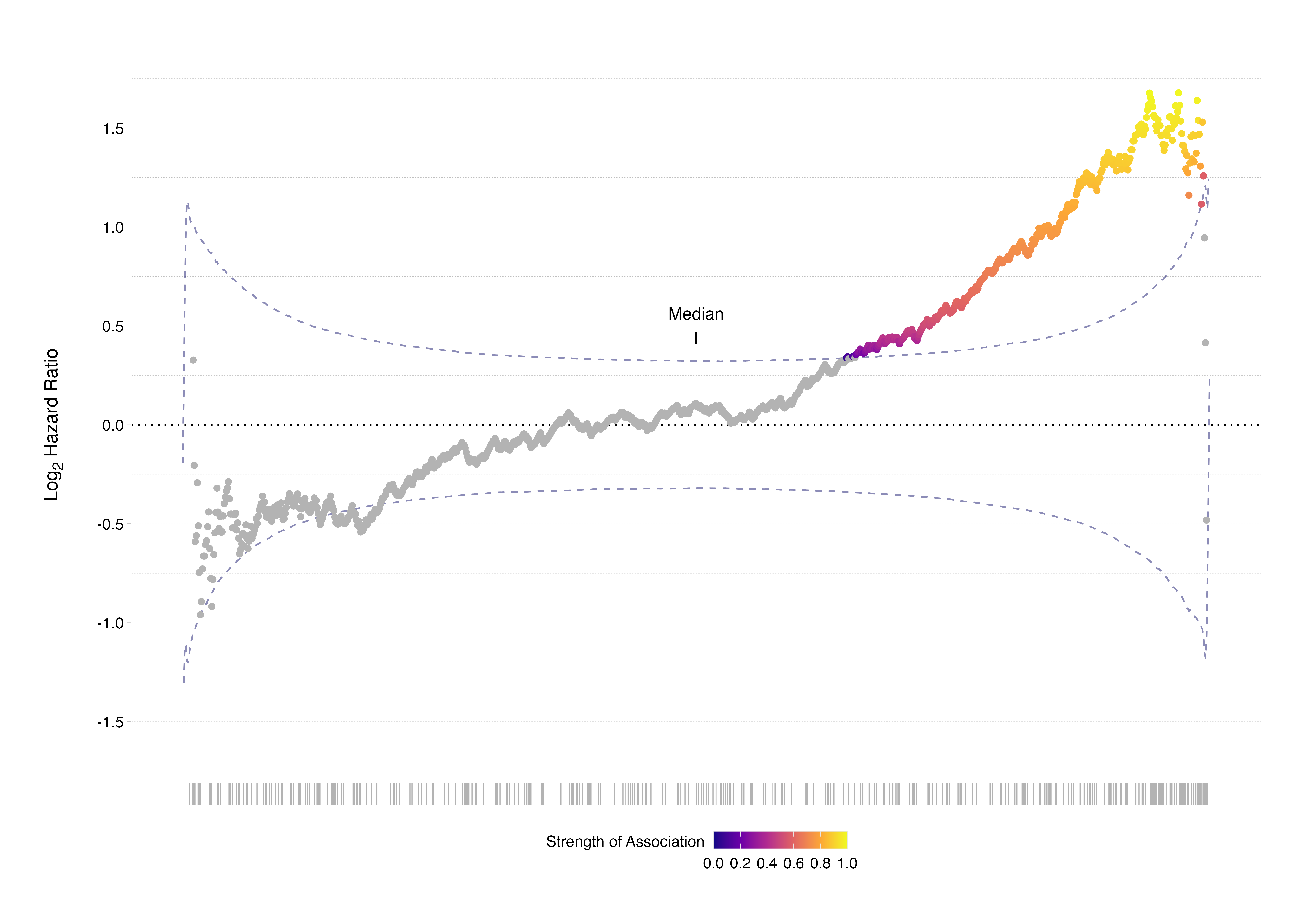 Source:
Naeemaee, R. et al. (2026) Innovations in Biomarker Stratification for Precision Oncology
Source:
Naeemaee, R. et al. (2026) Innovations in Biomarker Stratification for Precision Oncology
This example illustrates a critical and underappreciated truth: continuous biological systems rarely align themselves with arbitrary statistical quantiles. Molecular processes do not recognise medians, nor do they operate in compliance with evenly distributed group sizes. When we impose artificial thresholds without biological or statistical justification, we risk erasing real associations. In this context, the median split produces distortion not clarity.
For the benefit of those not up-to-speed on contemporary breast cancer therapeutics or open-access data sets, the reason that this example is particularly instructive is that ERBB2 encodes the protein HER2 - the therapeutic target of trastuzumab (Herceptin) - and METABRIC is widely recognised as one of the largest and most clinically representative open-access datasets in breast cancer.
The Illusion of Objectivity
The appeal of the median split lies in its appearance of objectivity. It feels impartial because it is mechanically determined by the data distribution. It appears free from researcher bias. Yet it remains one arbitrary cut among tens or hundreds of possible alternatives. Its neutrality is superficial.
The problem intensifies when researchers abandon the median in favour of searching for the “optimal” cut point. The minimum p-value approach, in which multiple candidate thresholds are tested and the one yielding the smallest p-value is reported, introduces a different but equally serious problem. Without appropriate correction for multiple testing, this strategy inflates Type I error rates. It effectively guarantees that some threshold will appear significant purely by chance, particularly in small or moderately sized cohorts.
What appears as a data-driven optimisation may, in fact, be an artefact of sampling variability. The selected threshold becomes dataset-specific and unstable. When applied to an independent cohort, it frequently fails to replicate. The apparent biological insight evaporates under external validation.
In small or heterogeneous datasets - precisely the conditions common in translational contexts such as clinical oncology - this instability is magnified. Both false negatives and false positives become likely. The issue is not that biomarkers inherently fail to validate. It is that the analytical strategies used to define their prognostic value often fail to respect the statistical structure of continuous data.
“Fine, I’ll Use Cox Regression”
In response to criticism of dichotomisation, many researchers argue that they are not relying solely on Kaplan-Meier curves. They use Cox proportional hazards regression and include the biomarker as a continuous covariate. This is unquestionably preferable to arbitrary categorisation. The Cox model accommodates censoring and estimates hazard ratios per unit increase in biomarker level. It preserves continuous information and avoids forced binary grouping. It also allows concomitant modelling of important clinical, pathological, and demographic covariates. Nice 👌🏻
The Cox model is not immune to misapplication. It also relies on assumptions that are frequently overlooked. First, the proportional hazards assumption requires that hazard ratios remain constant over time. In settings such as oncology, where treatment effects and disease biology can evolve dynamically, this assumption is often violated. Time-dependent effects, delayed therapeutic responses, or early transient benefits can all disrupt proportionality. Although formal tests such as Schoenfeld residuals are available, they are not routinely reported.
Second, the standard Cox model assumes a log-linear relationship between the continuous predictor and the hazard function. In biological systems, this assumption is rarely justified. Biomarker-outcome relationships can be (and frequently are) non-linear, plateauing, or even U-shaped (non-monotonic if you’re feeling fancy). If the true relationship deviates substantially from linearity, fitting a single linear coefficient across the entire biomarker range produces an averaged effect that may obscure clinically meaningful structure.
A non-significant hazard ratio under a standard linear Cox model does not necessarily imply absence of association but it may indicate model misspecification. Conversely, a significant hazard ratio may represent an averaged signal that lacks practical interpretability without understanding its shape.
There is an additional and frequently overlooked limitation of the Cox proportional hazards model in this context: even when correctly specified, it does not provide a clinically actionable threshold. A hazard ratio per unit increase or per standard deviation increase quantifies relative risk, but it does not tell a clinician where to intervene. It does not define a boundary between “treat” and “do not treat”. It does not specify a value at which risk meaningfully changes category. In other words, while Cox regression is powerful for inference, it does not, by itself, solve the translational problem that motivated dichotomisation in the first place.
This creates a tension in biomarker research. Investigators abandon arbitrary median splits in favour of modelling biomarkers continuously - which is statistically appropriate - yet clinical implementation often requires decision rules. Guidelines, reimbursement frameworks, and treatment eligibility criteria frequently demand categorical cut-offs. The danger, therefore, is a circular regression: researchers dichotomise prematurely for convenience, or they fit continuous models but later retrofit thresholds without sufficient validation. The statistical model becomes disconnected from clinical decision-making.
The solution is not to retreat to arbitrary splitting. It is to recognise that threshold definition is a separate and rigorous task. If a cut-off is required for clinical use, it must be derived transparently, validated independently, and justified biologically. The Cox model can describe risk gradients. It cannot, on its own, determine where biology ends and decision-making begins.
“Wait, So We Do Need Groups?”
In an ideal world, clinically actionable thresholds would absolutely exist. Clinical practice frequently requires categorical decisions. Treatment guidelines, reimbursement policies, and eligibility criteria are rarely written in terms of smooth risk gradients. They are written in terms of defined groups. The problem is not the existence of thresholds. The problem is how casually they are constructed.
If a biomarker is to guide treatment, its threshold should be derived from modelling that already accounts for the complexities we have outlined: non-linearity, confounding variables, cohort heterogeneity, time-dependent effects, and interaction with clinical covariates. A cut-off should not be the first analytical step. It should be the final translational step.
In other words, multivariate modelling should precede threshold definition. The biomarker’s effect should be evaluated alongside age, stage, comorbidities, treatment exposures, and other relevant variables. Its functional form should be characterised. Its stability across subgroups should be assessed. Only once its behaviour is understood within this broader framework should a threshold, if required, be proposed. Even then, that threshold must be validated externally and shown to retain clinical utility beyond the dataset in which it was defined.
A meaningful cut-off is not simply a statistically significant split. It is a decision boundary that survives adjustment, validation, and contextual scrutiny. Anything less risks rebranding convenience as precision.
The Problem is Forcing Biology into Boxes
At their core, the issues that I have bemoaned up to now extend beyond any single statistical method. The deeper problem is conceptual. Continuous biological phenomena are repeatedly forced into categorical frameworks because categorical outputs are easier to communicate. High risk versus low risk. Eligible versus ineligible. Treat versus do not treat. Binaries align comfortably with clinical decision-making structures.
Convenience does not justify distortion. When continuous biomarkers are dichotomised, gradient information is erased. Subtle dose-response relationships disappear. Cohort-specific thresholds masquerade as universal biological truths. Reproducibility suffers because thresholds derived in one dataset fail to generalise to another with slightly different distributions, treatment regimens, or patient demographics.
This pattern contributes to the high attrition rate of candidate cancer biomarkers. Many people in oncology research are somewhat familiar with the conclusions of Hernández and colleagues 2 (I know this because you hear the following banded around all the time); fewer than one percent of published cancer biomarkers ultimately reach clinical practice. While many factors contribute to this failure, methodological instability in threshold definition is undoubtedly one component.
“So, What’s the Solution?”
For most bioscientists conducting survival analyses, the solution does not require complex machine learning frameworks or advanced ensemble modelling. It requires methodological discipline.
Whether using Kaplan-Meier, Cox regression, non-linear splines, or more complex frameworks, two foundational steps are non-negotiable before any modelling decision is made: deep exploration of the dataset and critical evaluation of its representativeness. These are not optional preliminaries but prerequisites for meaningful survival analysis.
Extensive exploratory analysis is essential to understand the structure of the data: distributional properties of the biomarker, presence of skewness or multimodality, potential non-linear patterns, degree of censoring, event rates over time, missingness mechanisms, batch effects, and correlations with known clinical covariates. Without this groundwork, modelling choices become blind decisions. A threshold may appear unstable not because the biomarker is unreliable, but because the cohort is small, heavily censored, or structurally imbalanced. A linear term may appear insignificant because the true relationship is curved or restricted to a narrow range of values. Survival analysis is not merely the execution of a statistical function; it is an attempt to describe structure in noisy biological data. That structure must first be examined.
Equally important is contextual understanding of who the data represent. Contemporary oncology cohorts differ markedly in tumour characteristics, age distribution, ethnicity, comorbidity burden, treatment exposure, and in various other factors when compared with historical datasets. If the development cohort does not reflect current clinical demographics, risk estimates may not generalise. Apparent biomarker effects may, in fact, be confounded by demographic shifts or evolving treatment standards. Precision oncology demands not only statistical precision but demographic awareness. A biomarker that appears prognostic in a narrow or outdated population must be interpreted cautiously when applied to modern, diverse clinical settings.
In short, modelling sophistication cannot compensate for inadequate data understanding. Survival analysis should begin not with a p-value, but with a thorough interrogation of the dataset and the population it represents.
Continuous variables should, by default, be analysed as continuous. Non-linearity should be explored explicitly using flexible modelling approaches such as splines or smooth terms. Proportional hazards assumptions should be assessed rather than assumed. Threshold searching, if undertaken, should incorporate appropriate multiple testing correction and rigorous validation. If a clinically actionable threshold is genuinely required, it should be derived in one cohort and pre-specified for testing in an independent dataset.
So what’s the solution? Stop taking shortcuts. And most importantly, recognise that the statistical significance derived from a Kaplan-Meier split should not be equated with biological truth. A survival curve is a descriptive representation of grouped data. It is not, in itself, validation of a mechanistic relationship.
Precision Medicine Requires Precision Stats
Precision medicine promises treatment tailored to biological nuance. It aspires to move beyond crude categorisation and towards individualised risk assessment. However, if the analytical foundation of biomarker research begins by reducing continuous molecular measurements to arbitrary binaries, that promise is undermined at the outset.
The tools themselves are not the enemy. Kaplan-Meier estimators and Cox proportional hazards models are powerful and appropriate when used thoughtfully. The issue lies in the casual way they are applied, particularly when continuous biology is forcibly reshaped to suit categorical visualisation.
Survival models deserve respect, as do the biological systems they attempt to describe. When used carefully, they can illuminate meaningful patterns. When used reductively, they obscure them. Continuous biomarkers are not problems to be cut in half. They are signals to be modelled with care.
Our recent review paper Innovations in Biomarker Stratification for Precision Oncology in Clinical and Experimental Medicine discusses these issues in more technical detail.
Thanks for reading. I hope you enjoyed the article and that it helps you to get a job done more quickly or inspires you to further your data science journey. Please do let me know if there’s anything you want me to cover in future posts.
If this tutorial has helped you, consider supporting the blog on Ko-fi!
Happy Data Analysis!
Disclaimer: All views expressed on this site are exclusively my own and do not represent the opinions of any entity whatsoever with which I have been, am now or will be affiliated.